-
Convert Ancestry ProTools to Trees using AutoLineage and AutoKinship!
Genetic Affairs has unveiled a powerful new feature in AutoLineage—now you can apply AutoKinship to each individual cluster generated from Ancestry ProTools shared matches, unlocking a whole new level of insight into your family connections! It invokes the functionality of AutoKinship on the site directly at no additional cost, to provide reconstructed trees based on…
-
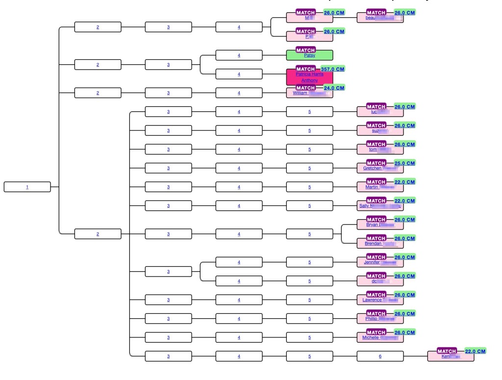
Pruning Your Trees in AutoLineage
I like to have pretty trees when I run ‘Find Common Ancestors’ on AutoLineage. But sometimes they turn out very messy. This blog will describe why that happens and how to fix it. The most common occurrence is when a match has more than one tree. I know that my second cousin (2C) Trish has…
-
Linking GEDmatch and FTDNA – AutoLineage for iGG
AutoLineage is a powerful tool that allows you to cluster your matches at a particular testing site but also to find common ancestors across multiple sites. In this blog, we will discuss a scenario when only data from FamilyTreeDNA (FTDNA) and GEDmatch can be used as sources, for instance for an investigative genetic genealogy search.…
-
AutoLineage
AutoLineage is the latest tool to be added to Genetic Affairs. It contains a number of the other tools, such as AutoClustering of DNA matches at any site. But the big new feature with AutoLineage is the ability to find most recent common ancestors (MRCA) for trees that you have added. These trees can be…
-
LivingDNA Chromosome Browser
The big news is that LIvingDNA finally has a chromosome browser. I’ve been waiting for this ever since we uploaded our DNA. You can see which segment on which chromosome you and your match share, but there’s no easy way to download the information. You can write it on paper and then copy to Excel…
-
Using MyHeritage Theories of Family Relativity
Recently MyHeritage announced some new, additional Theories of Family Relativity. Theories are similar to Through Lines on Ancestry, but they show all the pieces of the different trees that are used for the Theory. In a way that makes it a bit like a Quick & Dirty (Q&D) tree, only I didn’t have to make…
-
AutoSegment ICW Enhancement – Find Segments Linked to Opposite Parent Sides
Recently the AutoSegment ICW tool on Genetic Affairs for 23andMe and FamilyTreeDNA profiles has received significant enhancements. In short, if the DNA matches linked to overlapping segments are not shared matches (for FTDNA) or do not triangulate (for 23andme), it can be presumed that these segments are related on opposite parent sides. An AutoSegment analysis…
-
AutoKinship at GEDMatch
The AutoKinship tool was introduced on GEDmatch about a year ago. Developed by Evert-Jan Blom, AutoKinship is able to reconstruct trees based on shared DNA between shared matches. Genetic Affairs has AutoKinship for 23andMe data., as well as manual AutoKinship. Manual AutoKinship can be performed for any site that allows you to view the amount of…
-
RootsTech 2022
This year RootsTech will again be virtual and free! And it’s less than a week away!! You can register for RootsTech here. This year the conference is Thursday, 3 March through Saturday, 5 March. The Expo will open at 8 AM MST with the Expo Party! The first keynote speaker is at 10 AM and…
-
Subscribe
Subscribed
Already have a WordPress.com account? Log in now.
