Linking GEDmatch and FTDNA – AutoLineage for iGG

May 7, 2024 ~ Patricia Coleman ~ 6 Comments

AutoLineage is a powerful tool that allows you to cluster your matches at a particular testing site but also to find common ancestors across multiple sites. In this blog, we will discuss a scenario when only data from FamilyTreeDNA (FTDNA) and GEDmatch can be used as sources, for instance for an investigative genetic genealogy search.

An example reconstructed tree using only FTDNA and GEDmatch data.

We will be importing and analyzing data from FTDNA and GEDmatch, and use the common ancestor identification tool to find common ancestors. Also, we’ll show how to use the hints tool to get insights about ancestral lines that could hold a potential common ancestor.

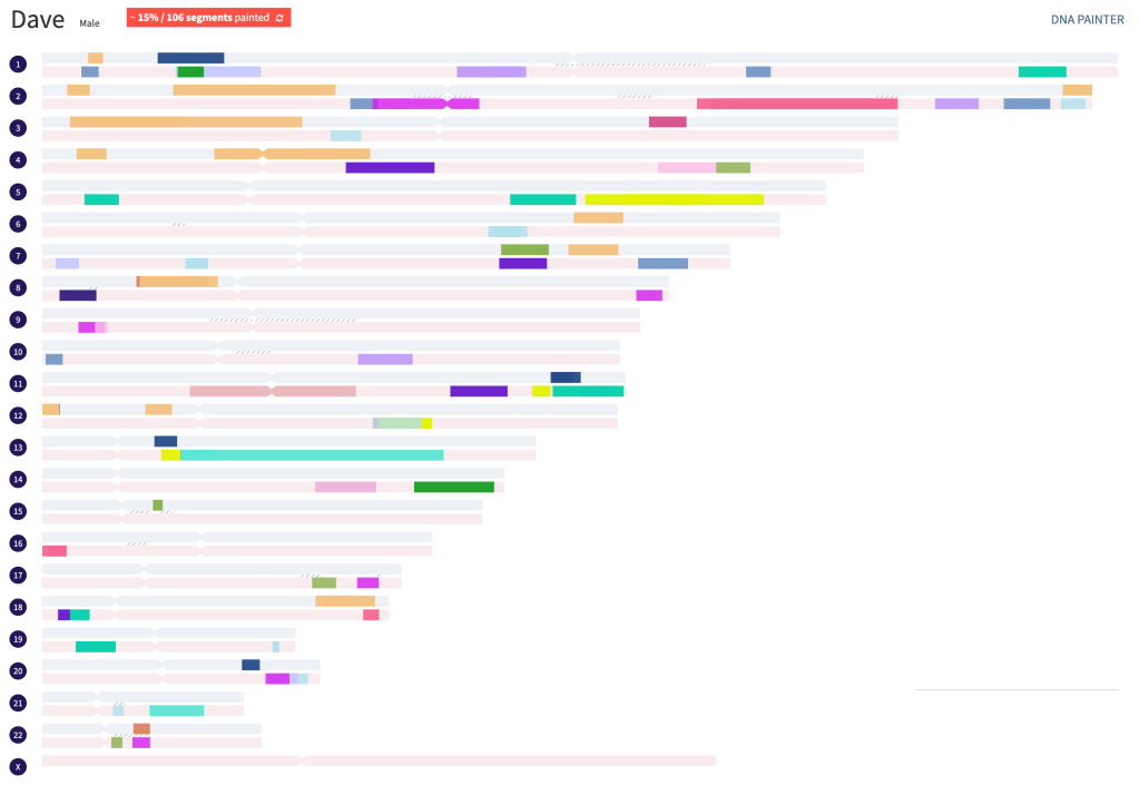
From the landing page select ‘Register a new Profile’ in the left panel. Start AutoLineage by making a profile for the case you are investigating and for whom DNA matches are obtained. In this blog, we shall be using Dave as an example.

Starting a new profile.

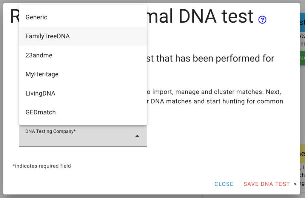
Family Tree DNA

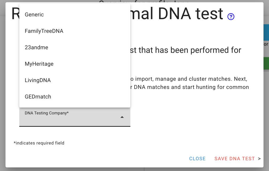
Next, a DNA test is registered.

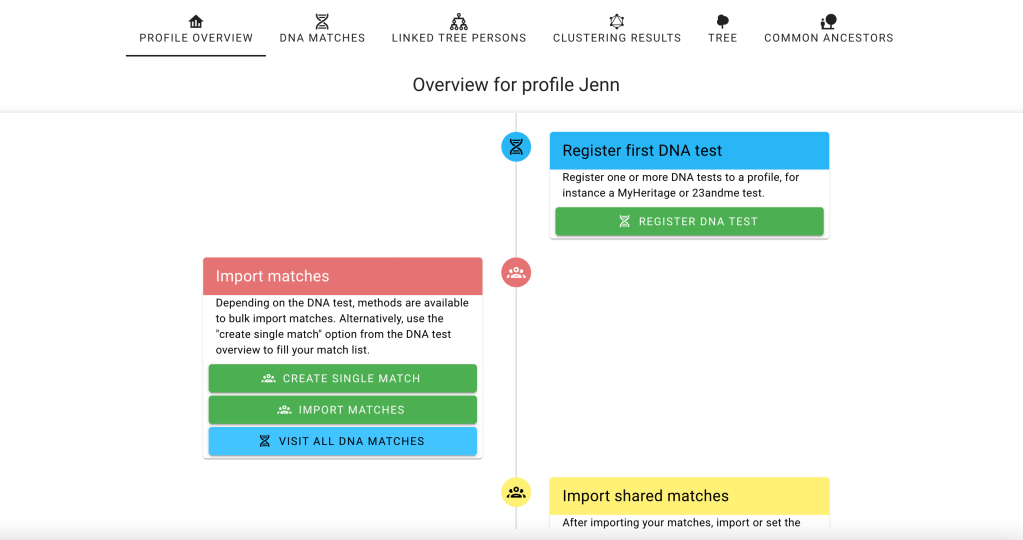
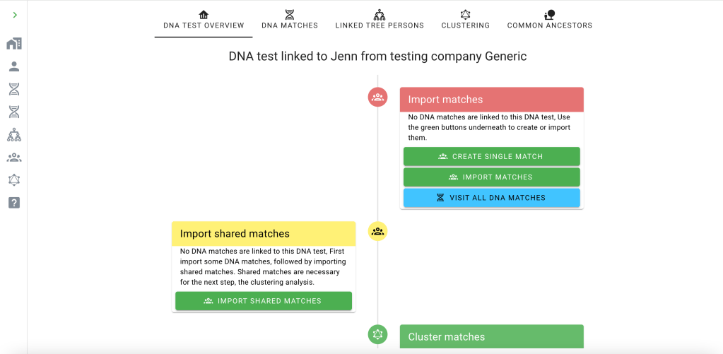
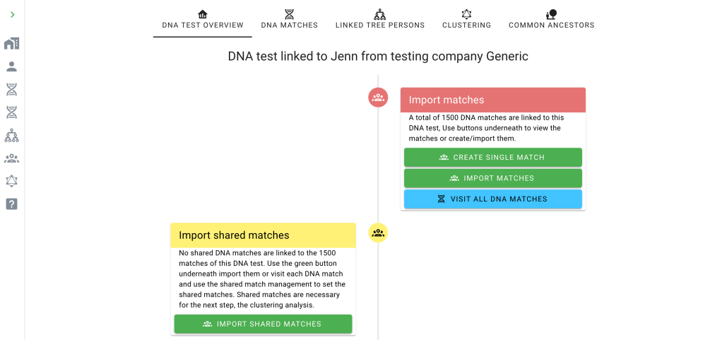
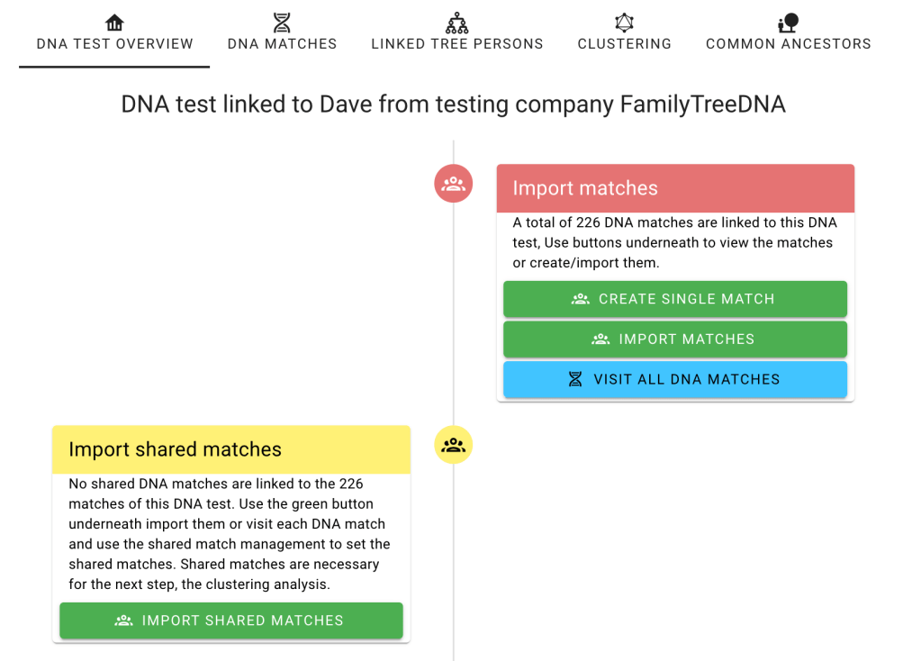
The first thing to do is to import Dave’s matches from FTDNA. Click on the ‘import matches’ button.

Flowchart showing Import matches.

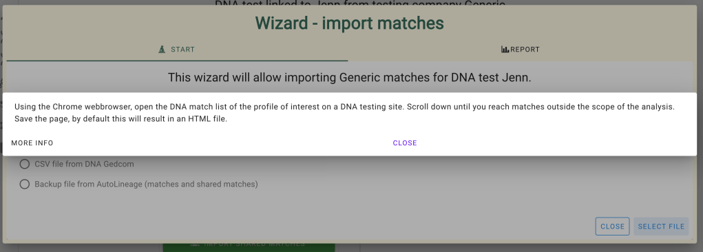
Each testing site has its own list of methods for collecting matches.

Options for uploading matches from FTDNA.

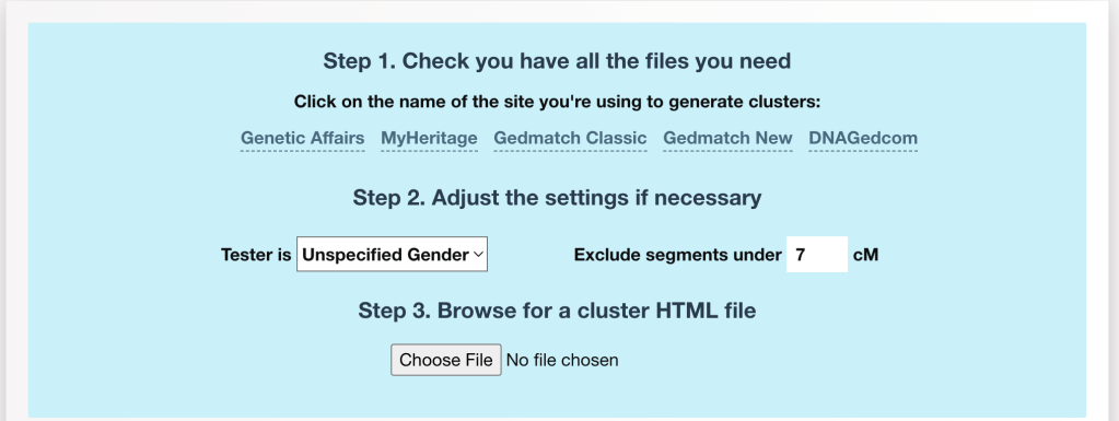
Here we are using the first one, a CSV file from Genetic Affairs. Clicking on the question mark explains what file this option needs.

Explanation of the CSV from Genetic Affairs.

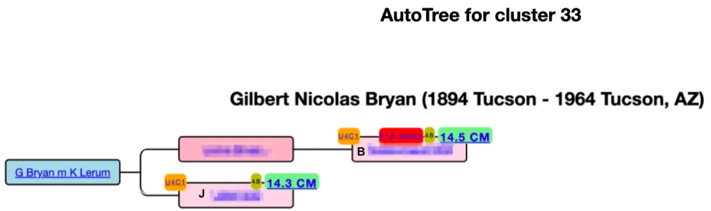
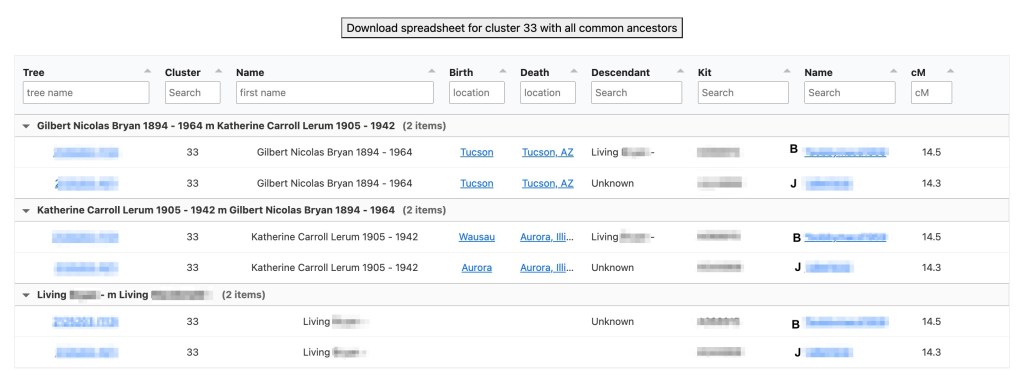
For this option, we first ran the AutoCluster analysis with the AutoTree feature enabled for FTDNA on Genetic Affairs.

Starting AutoCluster with AutoTree enabled on Genetic Affairs.

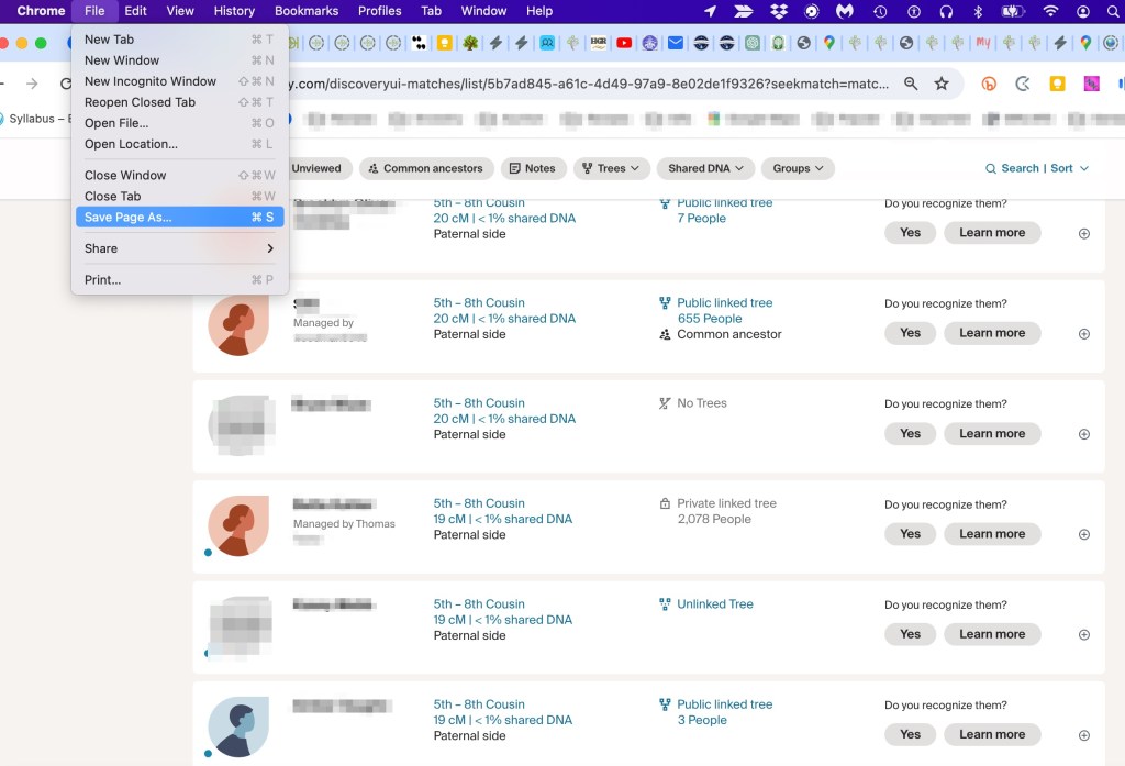
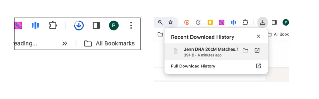
After starting the analysis, an email appeared with a download link. Alternatively, this link is also available in the notification section on the members page of Genetic Affairs (top right corner, under the bell icon).

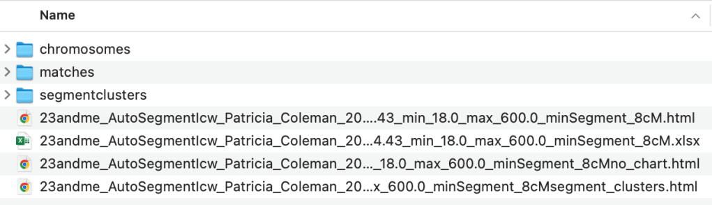
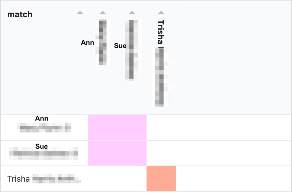
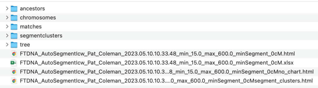
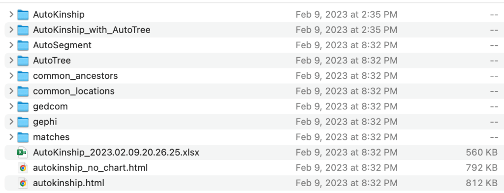
After unzipping the results file, we found all the data we needed for AutoLineage. In the Gephi folder, two files are present; nodes.csv and edges.csv. The nodes file contains the matches that would be selected in the dialog box of the ‘Wizard – import matches’.

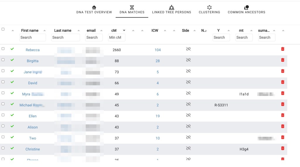
The imported DNA matches are shown after the import process has been completed.

Clicking on ‘DNA test overview’ at the top brought back the flowchart where we selected ‘Import shared matches.’. Shared matches are required for the clustering process.

The wizard explains that the edges.csv file from the Gephi folder is used for the shared matches.

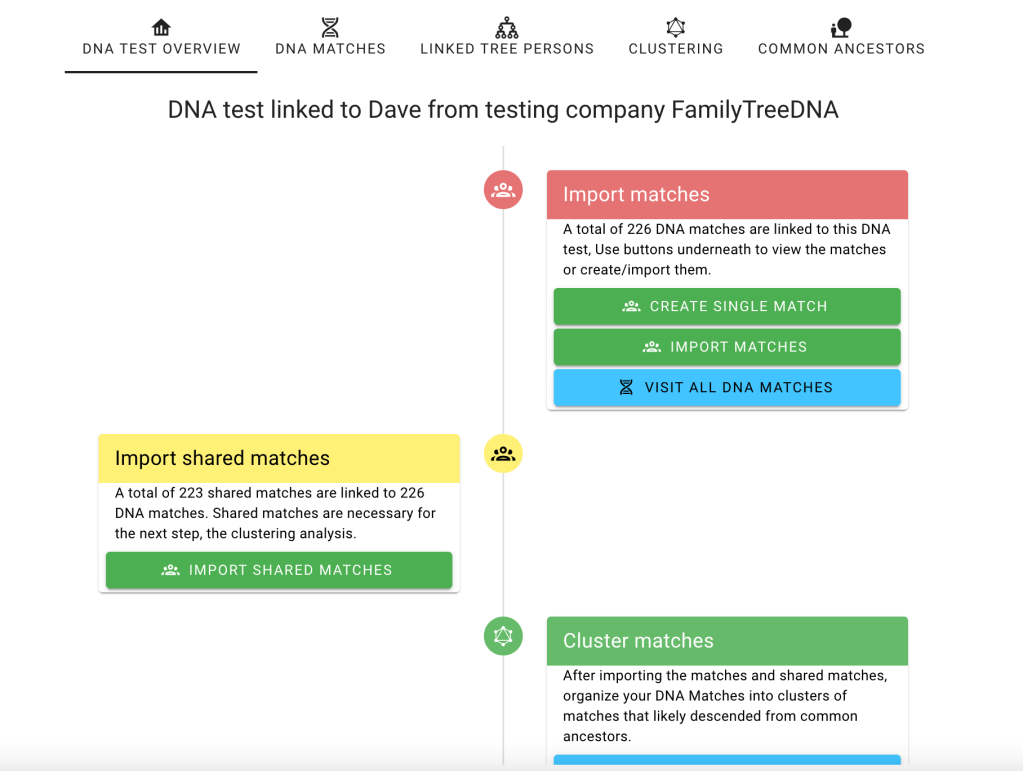
After importing the shared matches, which can take some time, the number of shared matches for each match is now displayed in the table.

Matches list showing the number of shared matches each has.

With matches and shared matches available, we ran the cluster analysis for FTDNA. Going back to the ‘DNA test overview’ brings up the flowchart where we selected ‘Cluster matches.’

The ‘Clustering wizard’ allows us to select the range of matches for the clustering, which type of clustering, and which color scheme should be used.

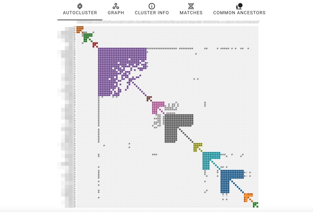
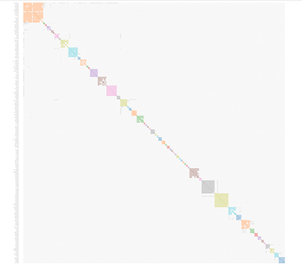
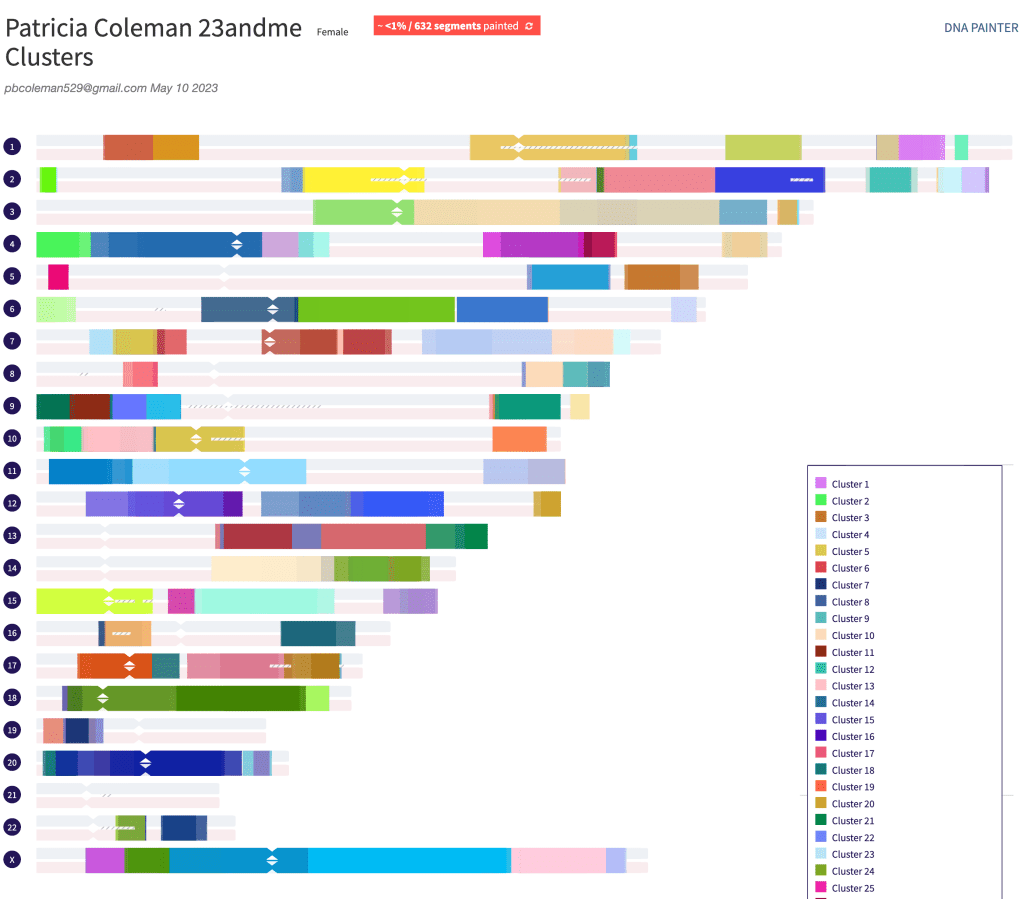
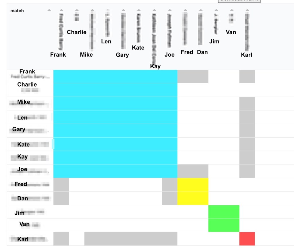
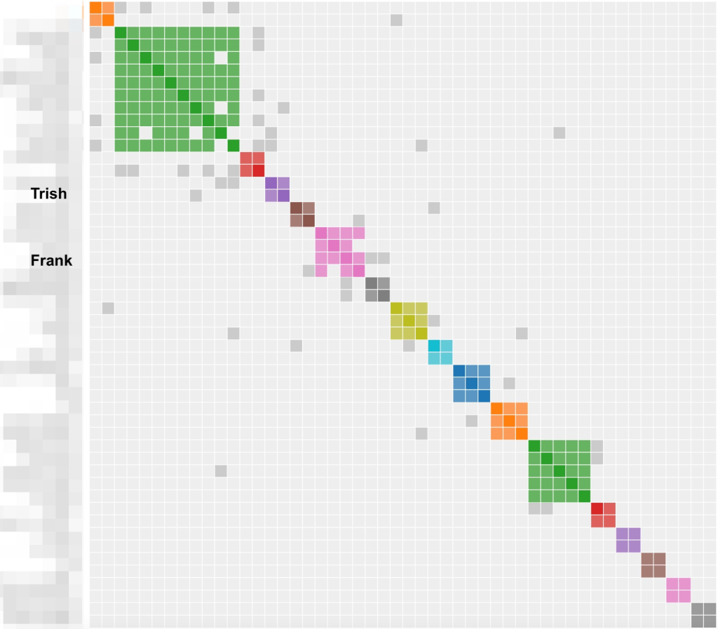
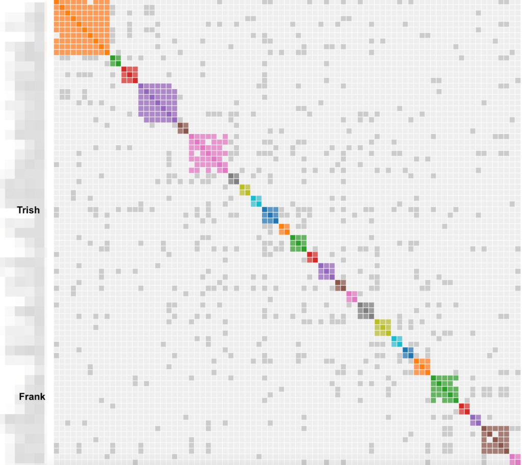
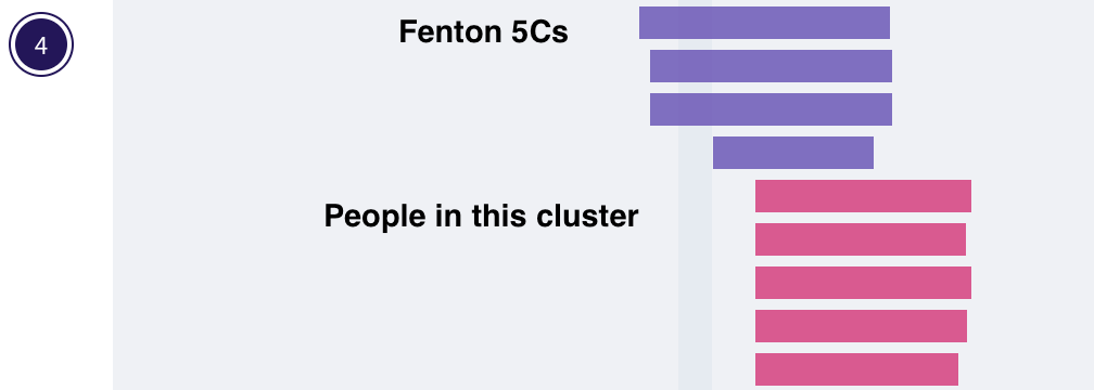
We selected to run all of Dave’s matches in the clustering analysis. After selecting the “start clustering” button, the clustering chart appears.

GEDmatch

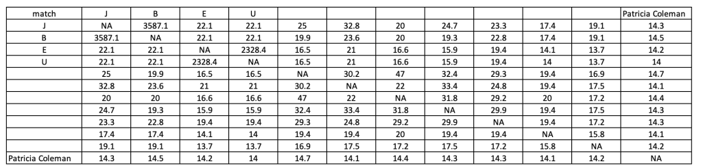
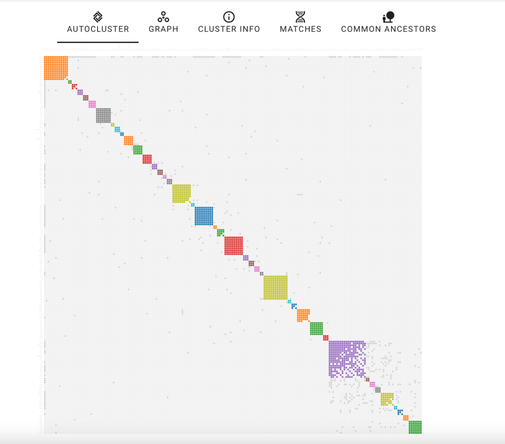
For the GEDmatch data, we added data from an AutoKinship analysis (Tier 1).

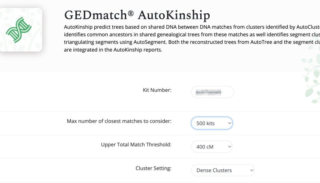
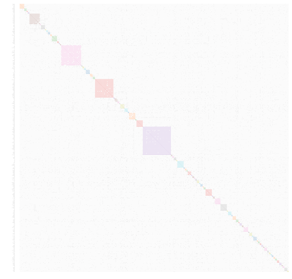
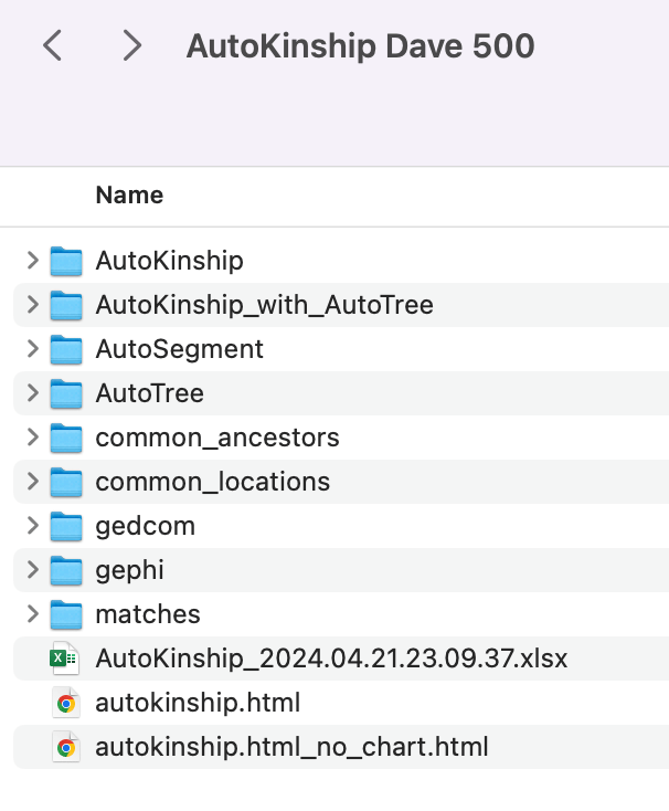
Going back to Dave’s profile page we registered another DNA test and selected GEDmatch from the drop-down list. Next we ‘import matches.’ An unzipped AutoKinship report also has a Gephi folder containing the nodes.csv and edges.csv files. Nodes.csv contains Dave’s matches, and edges.csv contains the shared matches. Now these matches can be clustered. We ran 500 kits for AutoKinship and 362 of these have shared matches.

Adding Trees

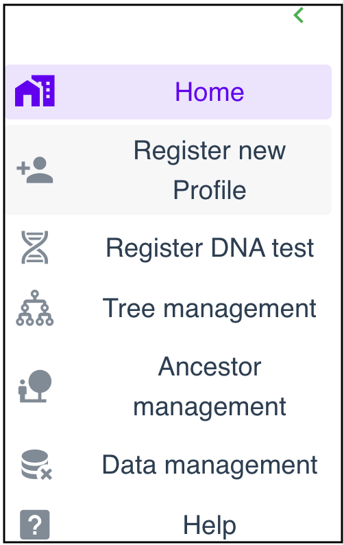
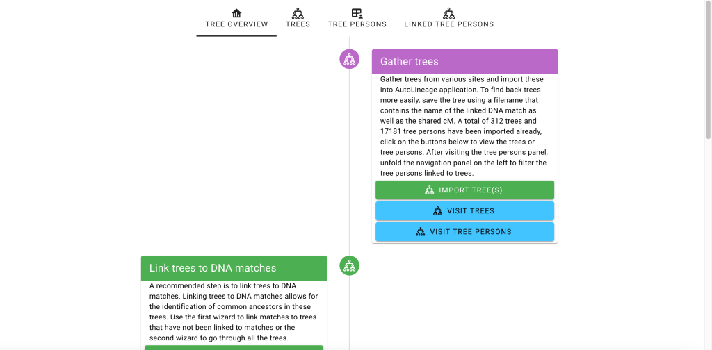
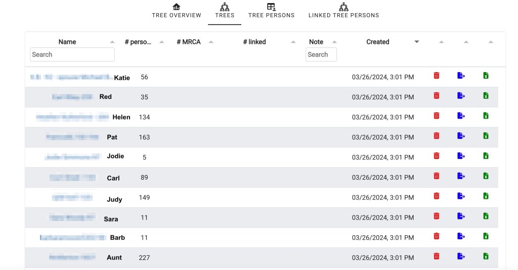
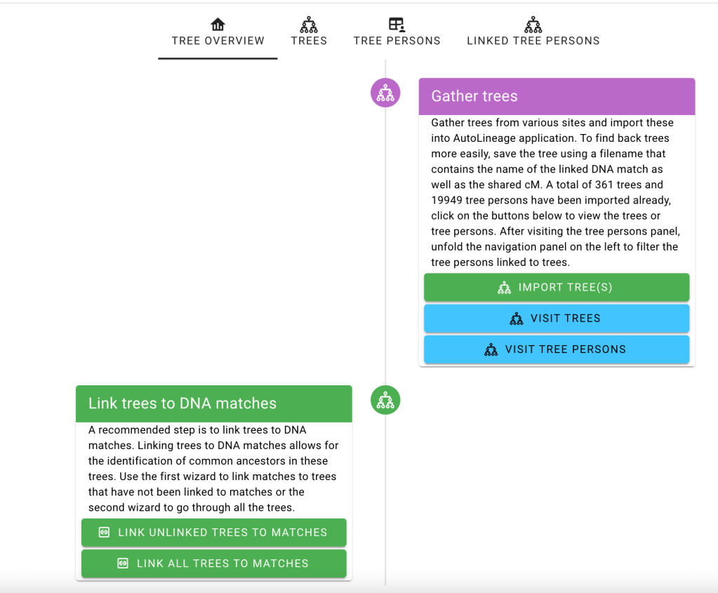
Now it’s time to add trees. The trees are typically associated with the matches, but they are managed independently of the DNA testing site. Clicking on ‘Home’ in the left panel brings up a list that includes ‘Tree Management.’ Clicking on ‘Tree Management’ brings up the flowchart for Trees.

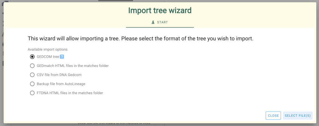
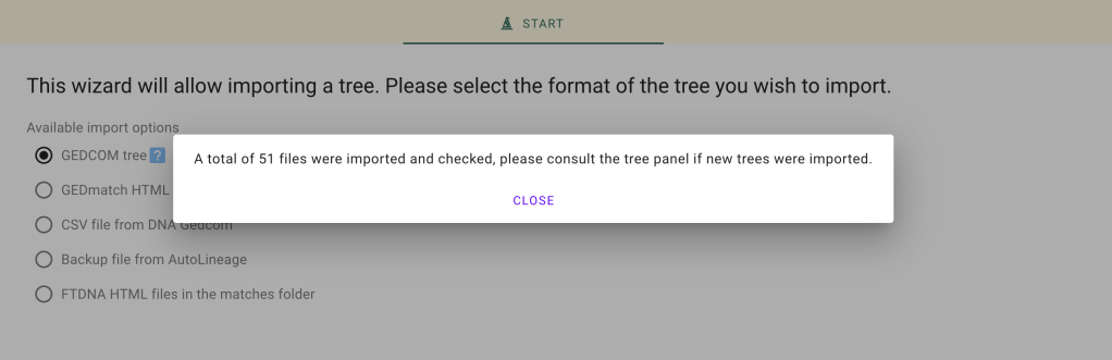
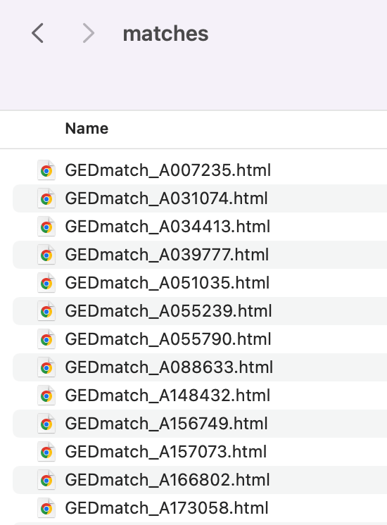
In ‘Gather Trees’ we clicked on ‘Import Trees’ which brought up the ‘Tree Wizard.’ There is a setting for the trees associated with the GEDmatch DNA matches, and a different setting for trees associated with the FTDNA DNA matches. In both cases, they retrieve tree information from the ‘match’ files associated with the GEDmatch AutoKinship or the FTDNA AutoTree AutoCluster.

‘Import tree wizard’ showing the two options for importing the trees associated with both testing sites.

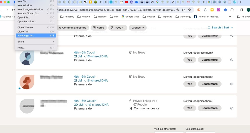
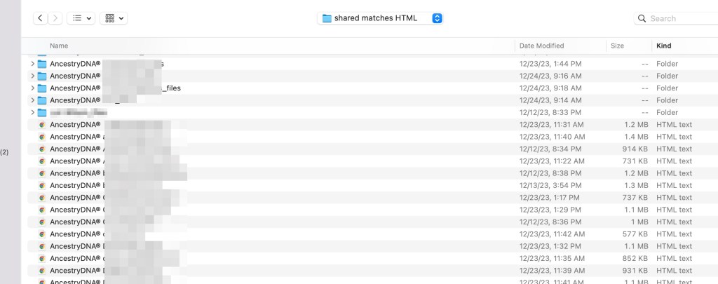
In both scenarios, we selected all the HTML files in the match folder of the unzipped AutoCluster FTDNA report or unzipped AutoKinship GEDmatch report. Using these methods also ensured that the trees were automatically associated with the FTDNA and GEDmatch DNA matches

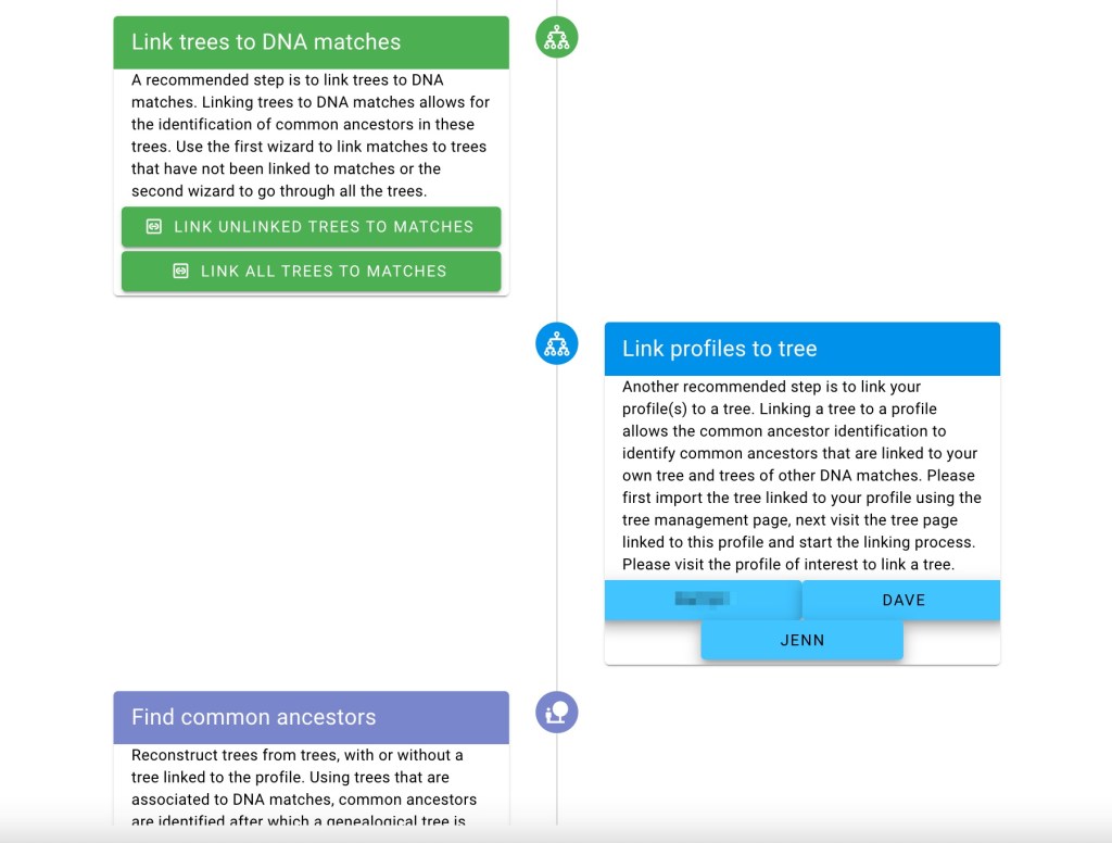
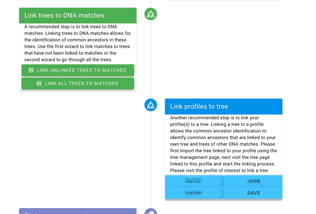
The GEDmatch AutoKinship folder contents.

The list of trees inside the matches folder.

Typically, iGG profiles are not associated with trees, but in our example, Dave does have a tree, and it needs to be linked to his profile. For other cases where the tester does not have a tree, such as people looking for birth parents, this step would be skipped, and you’d go on to ‘Find Common Ancestor’ from the various DNA matches.

To link Dave’s profile to a tree, we visited the tree management and select Dave in the ‘link profiles to tree’ section (alternatively, go to the tree view in Dave’s profile and associate the tree from there).

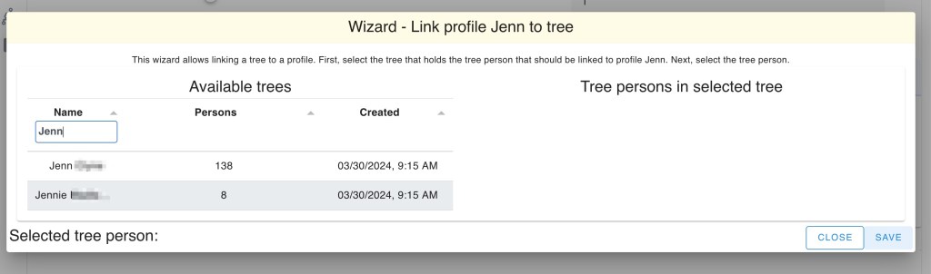
We clicked on Dave’s name and brought up the Wizard to link Dave’s profile to his tree. Next we searched for Dave’s tree in the name field.

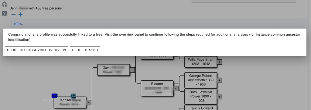
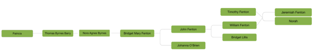
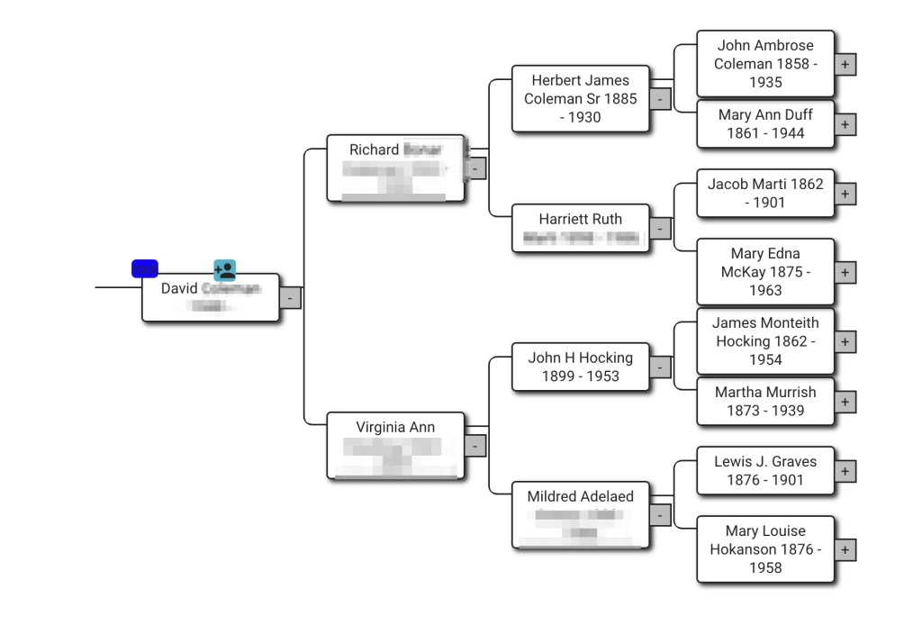
Selecting Dave brought up his tree where we selected him as the root person of the tree.

Selecting Dave as the root person in his tree.

This brought up Dave’s tree. Notice the person image over Dave’s name that tells the tree is connected to his profile.

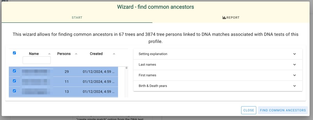
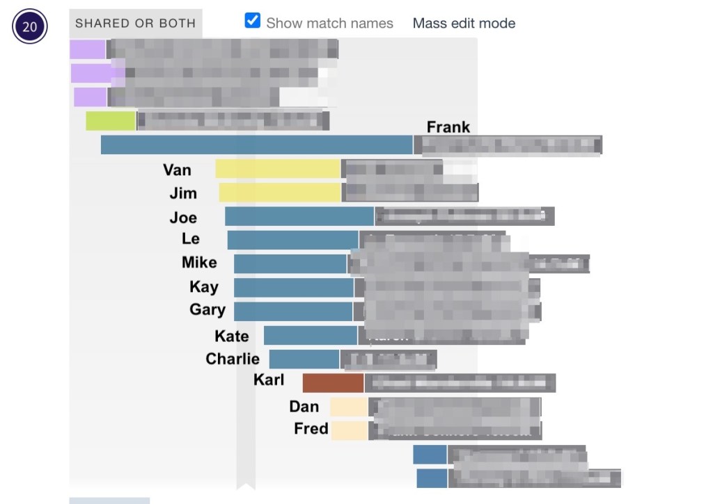
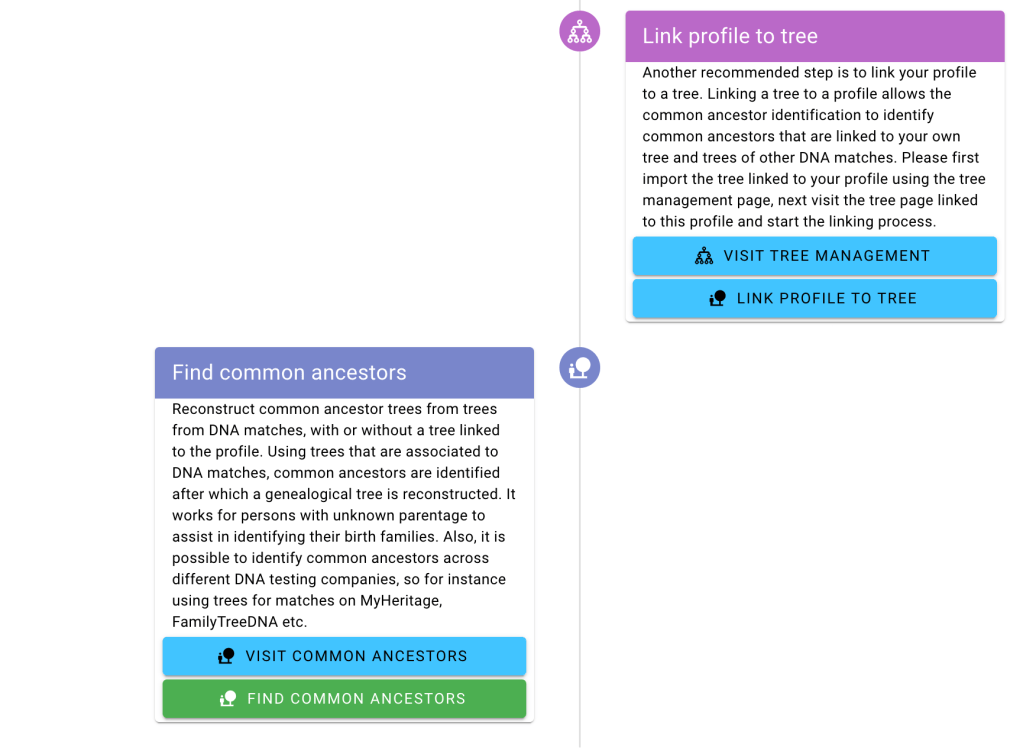
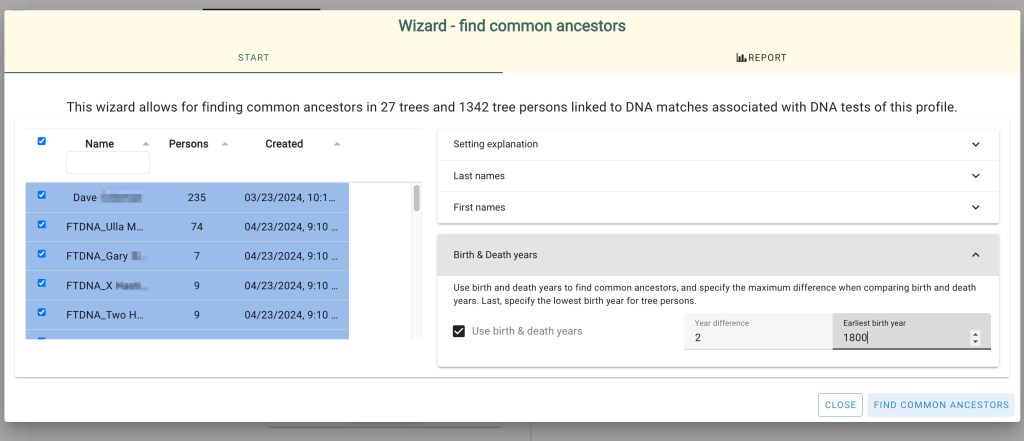
Dave’s tree. Names of living persons or those who died since 1973 have been hidden,

Going back to Dave’s profile page we scrolled down to ‘Find Common Ancestors’ near the bottom of the page. There are now two DNA tests associated to his profile, and some of the DNA matches are linked to trees that we imported. We selected the ‘find common ancestor’ button to start the common ancestor wizard.

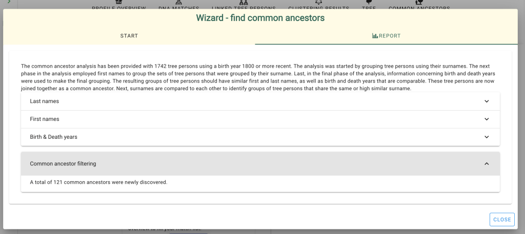
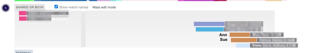
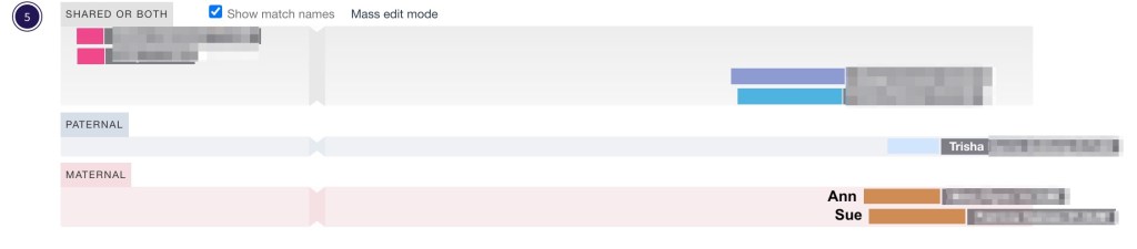
Running the analysis with the default birth year of 1800 identified eighty-seven common ancestors for Dave across FTDNA and GEDmatch. A problem arises when a match is on both sites and has a tree at both locations. The match on the right of the reconstructed tree shows both FTDNA and GEDmatch. She and her tree are duplicated which causes brown squares, indicating that tree persons are duplicated. Seeing a lot of these brown squares is often indicative of a problem.

DNA match who is on both sites and has trees on both.

Clicking on ‘Linked trees’ shows the trees that are attached.

Right-clicking on the tree brought it up in a new tab. Since the GEDMatch tree has more people we kept that one and deleted the FTDNA one. Next, we attached Rachel’s FTDNA DNA match to the remaining GEDmatch tree.

Connecting Rachel’s FTDNA match to her GEDmatch tree.

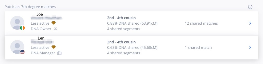
Rachel shared 30 cM with Dave at FTDNA and 27.7 cM at GEDmatch. Looking through the list of matches in the Wizard there’s only one Rachel that matches Dave at FTDNA with 30 cM, so we selected that one.

Clicking on the DNA symbol over Rachel’s name shows she is connected to both GEDmatch and FTDNA matches to Dave.

Finding Hints

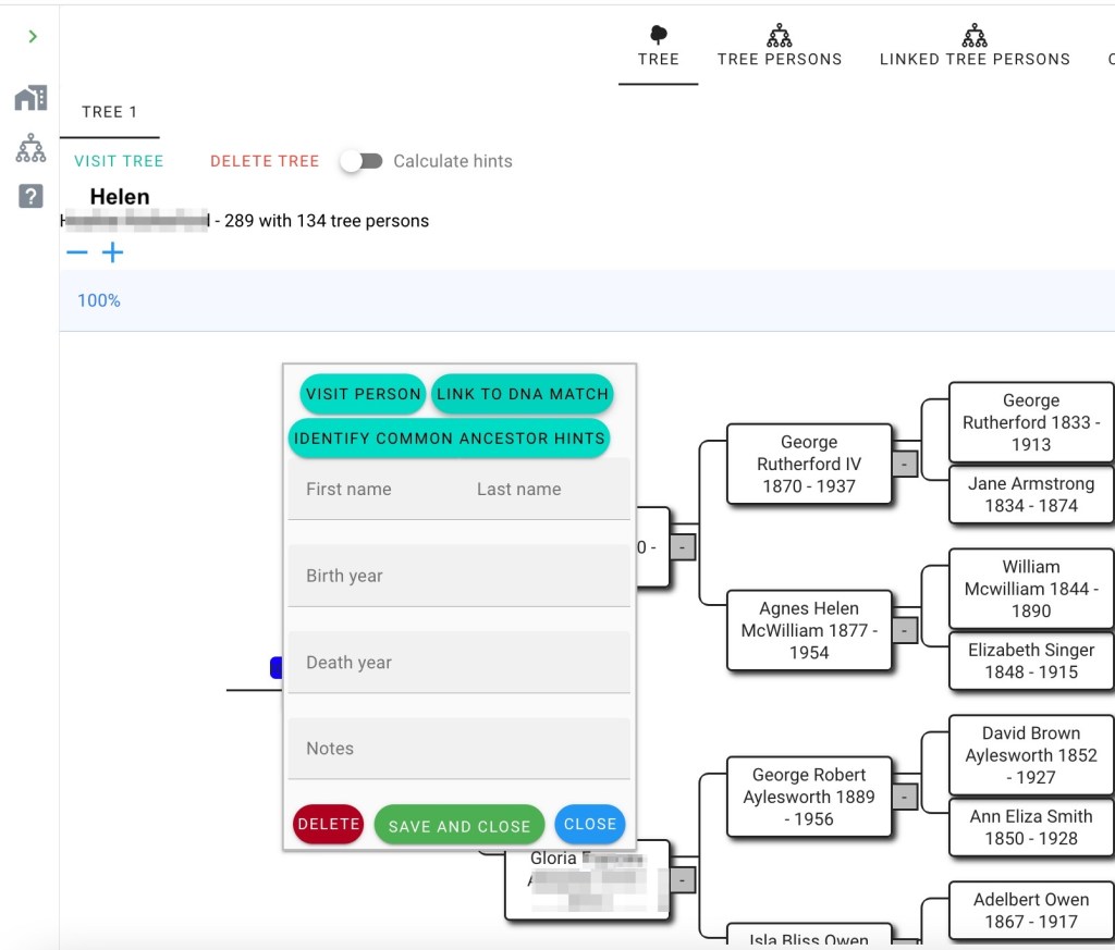
Since Rachel was the only match on both FTDNA and GEDmatch we used her tree and ‘calculate hints.’

Calculate hints is basically a common ancestor identification with a focus on the tree that is shown on the screen. The tool compares the names and dates in Rachel’s tree with all the other trees that have been loaded into AutoLineage. It can take a minute or so for this calculation depending on how many trees there are. Contrary to the regular common ancestor tool, the hints tool also shows hints about shared surnames and/or surnames and first names.

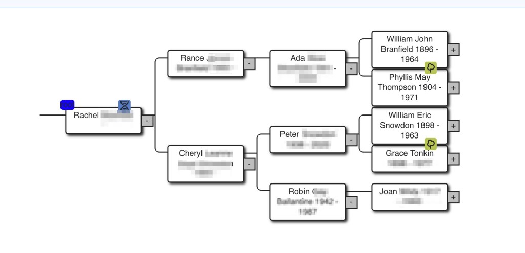
The calculate hints from Rachel’s tree showed a yellow hint for Phyllis May Thompson and for Grace Tonkin. Yellowish hints indicates a shared surname and might mean that there might be something useful farther back in time. So we expanded the tree out first from Phyllis. The common surname, Barrett, was found in another DNA match’s tree, but the dates were several hundred years different. Next we looked at the hint for Grace.

Grace Tonkin’s hint showed that Dave had several people in his tree with the Tonkin surname, but her date is more recent than the people in Dave’s tree. We followed the Tonkin line past Grace in Rachel’s tree and found that Thomas Tonkin’s dates were in the same range as those in Dave’s tree.

Thomas Tonkin’s wife, Margaret Hattam, also has a hint.

Looking at Margaret Hattam’s hint we find that Dave’s tree has several Hattam ancestors.

Margaret Hattam was born in 1785 and Dave has an ancestor, Mary Hattam born in 1783. When we added Margaret’s parents to our tree, and rerun the hints tool we found new green hints linked to Margaret’s parents.

John Hattam and Elizabeth Eddy both have green hints.

Looking at John Hattam’s hint we found that he is in both Rachel’s tree and Dave’s tree. We’ve found the common ancestor!

John Hattam in both Rachel’s and Dave’s trees.

Since John Hattam had a birth date of 1754, we changed the birth year to 1700 in the parameter of the ‘Find Common Ancestors’ wizard and then reran ‘Find Common Ancestors.’

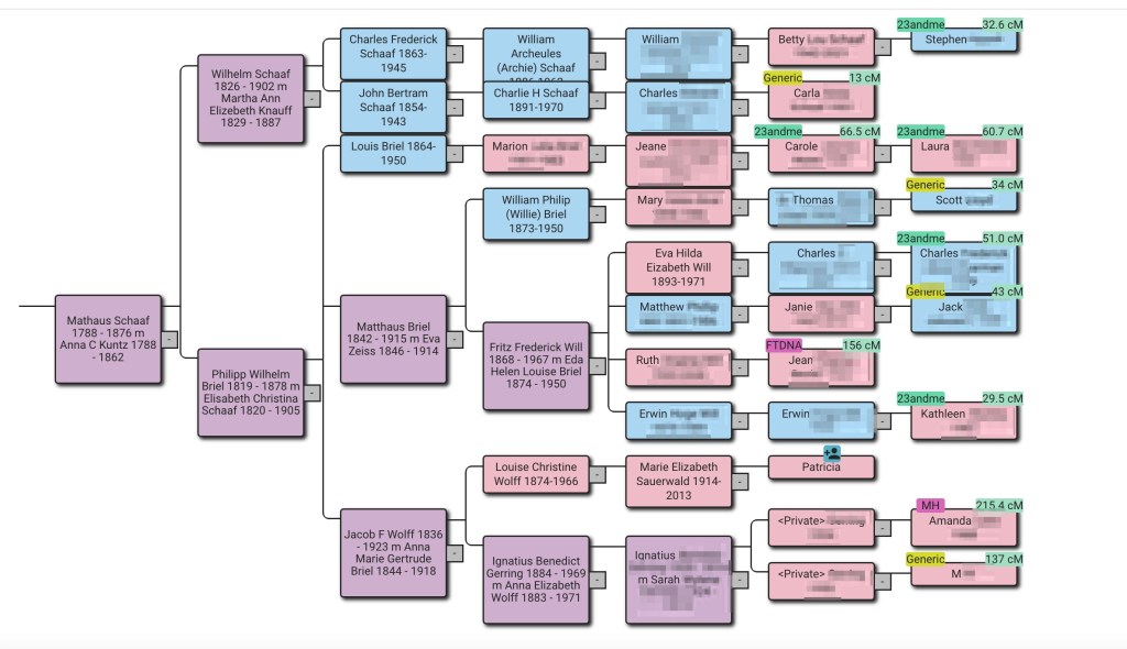
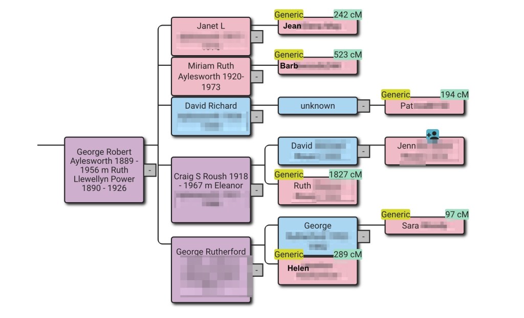
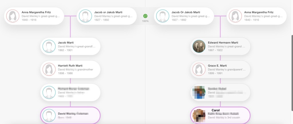
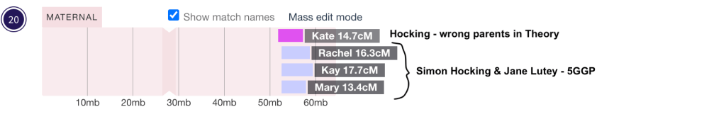
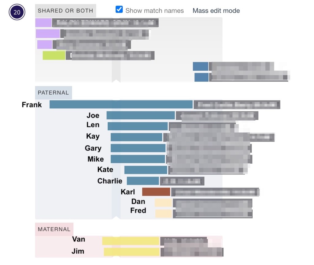
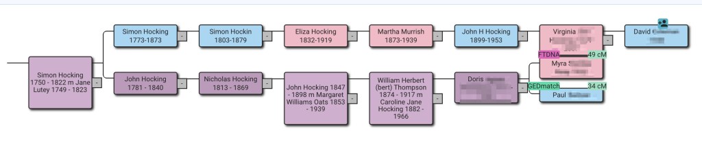
Changing the birth year in the Find common ancestor Wizard.

Now a total of fifty-four ancestors were found, and the reconstructed tree showed the connection between Dave and Rachel. They have common fourth great-grandparents, John Hattam and Elizabeth Eddy.

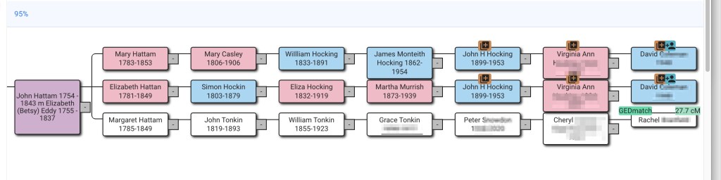
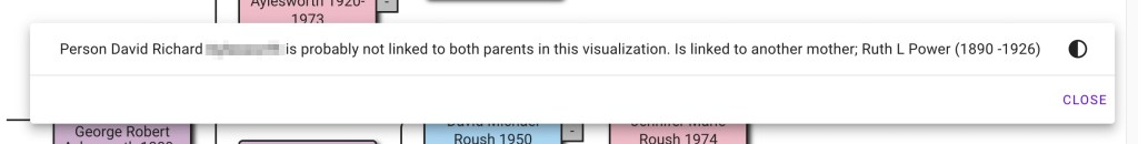
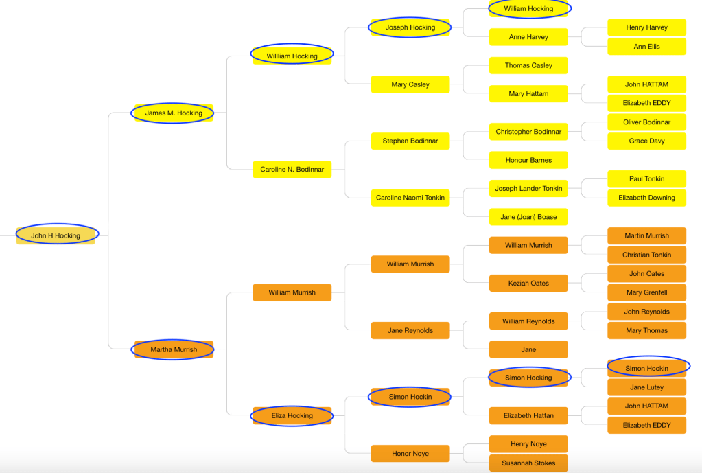
Reconstructed tree connecting Dave’s and Rachel’s trees.

Dave’s tree is showing brown squares which often means there is a duplicate tree or a date problem, however for Dave’s family this is correct. He has two Hocking lines. John Hocking’s parents were James Monteith Hocking and Martha Murrish. James Monteith is one of the Hocking lines, and Martha’s mother was Eliza Hocking, which is the other Hocking line. They both go back to John Hattam and Elizabeth Eddy, so they are Dave’s fourth great-grandparents twice!

Summary

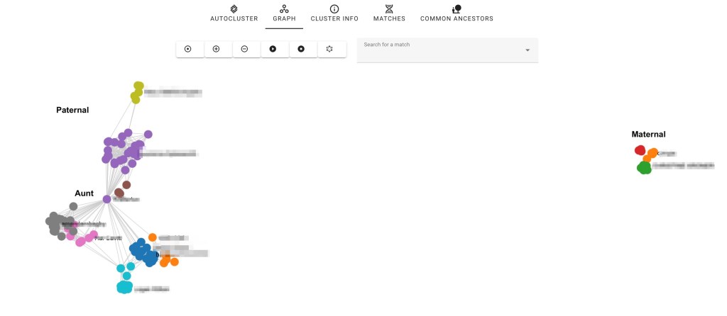
We ran AutoLineage using only FTDNA and GEDmatch data to look for common ancestors to Dave and his matches. AutoLineage generated clusters for the FTDNA matches and also for the GEDmatch matches. Trees from both testing sites were loaded and attached to the DNA matches. Next, we identified common ancestors across all of the data. We found one match who had a tree on both sites. By associating her DNA from both sites to one tree and deleting the extra tree we avoided her showing as a common ancestor to herself. Next, we ran hints on her tree to get clues on which ancestral lines to prioritize for our research. After expanding the tree, and re-running the hints tool, we found the common ancestor. This led us to find that she and Dave had common fourth great-grandparents!

AutoLineage

March 24, 2024August 6, 2024 ~ Patricia Coleman ~ 4 Comments

AutoLineage is the latest tool to be added to Genetic Affairs. It contains a number of the other tools, such as AutoClustering of DNA matches at any site. But the big new feature with AutoLineage is the ability to find most recent common ancestors (MRCA) for trees that you have added. These trees can be connected to DNA matches from any of the sites you have entered. I’d not realized how many of my cousins had done DNA tests until AutoLineage generated this reconstructed tree for my second great grandparents, Mathaus Schaaf and Anna Kuntz. This tree was generated using eleven trees of DNA matches and my tree. Where each DNA match tested is given as well as the amount of centimorgans we share is listed along with the match’s name. The surnames of living people as well as anyone who died after 1973 is hidden.

Getting Started

The first thing is to define a Profile for the person who has taken a DNA test. This might be you or another family member that you’re helping. I’m going to use my daughter, Jenn, for the test taker in the examples. On the left panel select “Register a new Profile.”

The left panel of AutoLineage.

The following dialog box appears where you enter the name of the tester.

Now the new profile is added to the list.

AutoLineage list of profiles, DNA tests and MRCA.

Next clicking on Jenn’s name in the list brings me to the ‘Profile Overview’ page where I can add a DNA test to her profile.The flowchart leads me through the steps. First I click on ‘Register DNA Test.’.

The ‘Register Autosomal DNA test’ page has a menu of the testing sites that AutoLineage supports.

Menu for selecting Autosomal DNA testing Company.

After selecting Generic from the list and clicking on “Save DNA Test,’ the “DNA Test Overview’ page shows the next step is to obtains Jenn’s matches.

DNA Overview page showing Import matches as next step.

Clicking on ‘Import Matches’ brings up the Import Wizard which shows several choices for Generic.

HTML file saved is selected which puts the blue question mark next to that selection. Clicking the blue question mark provides the explanation for obtaining that data.

To get the matches for Ancestry in HTML format, I visit Ancestry and click on Jenn’s DNA matches.

I want to collect Jenn’s data down to 20 cM so I’ll use the scroll bar on the right of the window and go to some value below 20 cM. Alternatively I could have selected the range for ‘Close matches’ to only go to 20 cM.

Select Close matches to only go to 20 cM in the match list.

Once I have Jenn’s match list down to 20 cM I’ll select ‘Save page as.’ from the Chrome File menu.

Save Page as to save the HTML file of all the matches down to 20 cM.

While the file is downloading you do not want to leave the page. There’s a symbol in the upper right of the Chrome page that shows a circle and an arrow. The circle around the arrow fills as the file is downloading. When the download is complete it changes to the arrow with what looks like an inbox under it. At that point the download is complete and it will show the filename. Then it’s safe to leave the page. This save will be an HTML file and a folder with a bunch of files in it. Apparently, the HTML file needs all these others, because if you delete the folder, the HTML file will not work anymore.

On the left the symbol as the file is downloading. On the right how the symbol looks when the download is complete.

Then going back to AutoLineage and the Wizard to upload matches, click on Select File, and then click on Jenn’s Data 20cM HTML file.

Once the data is received at AutoLineage the Wizard reports how many matches it found.

Wizard showing how many matches were retrieved for Jenn.

Once the wizard is closed the list of DNA matches appears.

The list shows how many cM the match shares with Jenn and which side of the family the match is predicted to be on. I have very few close cousins, so having all the of matches, except me on Jenn’s paternal side makes perfect sense to me.

Next I can add shared matches for her list of matches. He aunt and Barb, who is a 1C1R will match many of her DNA matches, so I’ll start with Luke since he’s just below 400 cM. I go back to ‘DNA Test Overview,’ and can select ‘Import shared matches.’

DNA Test Overview to ‘select’ Import shared matches.’

The ‘Import shared matches’ wizard looks very much like the import matches one. Here you can select all of the shared matches at once. Again go back to the test site and visit the match of interest and their shared matches.

Once again I scroll down to the bottom of the list of shared matches and select ‘Save Page As.’

Again wait for the little symbol to show that the file has been downloaded.

Luke’s shared matches saved to folder of Jenn’s shared matches.

Depending on how far down in cM you want to run your analysis collecting all of the shared match data for every DNA match can be time-consuming. But then it’s all there on your computer and you can run whatever range of cM that you choose.

I sort my list of matches by file type which I find makes it easier to add all the shared matches HTML file at one time.

Shared match list ready to be uploaded to AutoLineage,

After saving the shared match HTML files for all DNA match, go back to the import shared matches wizard, and select all HTML at once. While the shared matches are being added to AutoLineage the Wizard will often give a message about what it’s doing.

Import Shared matches Wizard adding shared matches files.

When all the files are added the Wizard will give a message about what it has found.

There were 47 files of shared matches with 5304 matches retrieved,

Now the ‘DNA matches’ has been updated to show the number of shared matches each match has.

Going back to “DNA Overview’ shows that running a cluster of these matches is the next item available.

On the ‘DNA Overview’ page ‘Cluster matches’ is the next item.

To get clusters for Jenn’s data that has been added, I’ll ‘perform clustering analysis.’

As you can see there are several different options. A Leeds-type analysis can be run using the matches from 400 to 90 cM, or a cluster using all the data can be run. If all the data is used, it can later on be reduced to view only 400 to 90 cM without rerunning the cluster. Different types of clustering algorithms can be used. ‘Normal’ is the type of cluster usually seen from the various software packages. Also, different color schemes can be used.

Not surprisingly the match in the purple cluster who matches almost all the others is Jenn’s paternal aunt.

Now I can take that cluster and change the range of matches that I want to see by changing the min and max number of cM..

cM range selector for the cluster display.

New clusters for 400 to 90 cM after adjusting the cM range,

At the top of the page for the AutoCluster are some other options. Clicking on ‘Graph’ brings up a Gelphi type display.

The ‘Graph’ display for Jenn’s 90 to 400 cM AutoCluster.

The majority of Jenn’s matches are paternal. I’m an only child and my closest cousins are second cousins. Several of them share DNA with Jenn, but not many whereas she has a lot of paternal cousins who show up in her matches.

‘Cluster info’ allows you to add any comments you want for the cluster. ‘Matches’ provides more details of the matches in the cluster. It has the matches’ names, the cM, the color of the cluster that contains that match, the number of ICW (In Common With) matches, which side of the family where the match is located and the cluster number, I’m in the first, orange cluster. In the green cluster is my second cousin, Patricia Harris Anthony, who has given permission to use her real name, At this point we’ve not found ‘Common Ancestors.’

Next selecting ‘Home’ from the left panel and then ‘Jenn’ for profile and scrolling down the next item on the flowchart is to gather trees.

Trees do not depend on the DNA site where a match has tested, For example, if someone has tested on several different sites their tree would not be different from one site to another. They might have a larger tree on one site than another but only one tree is needed to identify their family. Ancestry and MyHeritage seem to be the sites that have the most family trees. FamilyTreeDNA and GEDmatch have a smaller number in comparison. Clicking on ‘Gather Trees’ takes us to the ‘Tree Management’ page and flowchart.

Clicking on ‘Import Trees’ bring up the ‘Import tree wizard,’ which gives several choices for trees partly depending on where the match’s DNA data is located.

Again there is information on how to get the GEDCOM trees at the blue question mark.

Wizard explaining how to make gedcom images for trees.

One2Tree is a Chrome extension provided by NordeboApps Handelsbolag. A free version will give you four generations, but many trees are larger than that and depending on your family, you’d want to be able to go farther back than that. A subscription to One2Tree is 79 SEK (Swedish Krona) which is currently $7.48 US dollars.

Jenn’s highest match under 400 cM was Luke, but he does not have a tree. Moving to her next match, Helen, she does have a tree. Helen has three different unlinked trees, After looking at them we find the one that connects to Jenn’s family,. Clicking on her tree brings up another tab. You might have to go from the shared match page to ‘expand tree’ and then right click to get the detailed tree. Change the tree into ‘horizontal’ view and then use One2Tree from the Chrome extension to save the gedcom.

Once you have One2Tree installed as one of your Google extensions it will be shown in your list of extensions. Select it and the program will appear allowing you to save a gedcom of the tree.

After selecting One2Tree a dialog box appears asking if the person whose pedigree is shown is male or female. This one is for Helen, so I selected female,

Clicking on ‘Ok’ saves the file to my Download folder with filename One2Tree. Then I rename the file with Helen’s name and shared cM and move it to a folder of gedcoms for Jenn. When matches, like my second cousin Patricia Harris Anthony, match several of us, I have another folder for more general gedcoms. I know that none of Jenn’s paternal matches match me, so I keep them in her gedcom folder. This is my method for avoiding more than one gedcom for any match,

Just like with collecting shared matches, now I go through the match list and generate gedcoms for all the matches. Next they are added to AutoLineage with the ‘Import Trees Wizard.’

Fifty-one trees were found for Jenn’s matches.

After closing the Wizard the list of trees appears.

Clicking on ‘Tree Overview’ brings up the flowchart for trees.

There are two options to link the trees. If you are setting up trees for the first time either option will give the same results. If you’d already linked some trees and want to link new ones that you’ve just added, select ‘Link Unlinked Trees.’ Since you only one copy of a person’s tree in AutoLinage, when a match has tested at more than one of the testing sites, use ‘Link All Trees’ to add additional DNA matches to the existing tree.

The Wizard to link the root person of Haley Jones’ tree to her DNA match.

The Wizard added Haley’s picked up Haley’s first name and then found all DNA matches with first name Haley. I’ve found if the first name doesn’t bring up the correct match, delete it and put in the last name. For example, if a match used an initial and a last name, the initial might bring up a long list, and searching with the last night would be faster. Sometimes there may be a long list of DNA matches and the match’s name is not shown. There is a slider to the right of the window that lets you easily move down the list.

Slide to move down the list of matches if the name you’re looking for is not shown.

Alternatively, the DNA match can be linked to the tree from the ‘Tree’ page by clicking on one of the DNA matches. Here I clicked on Helen in the tree list, which brings up her tree. Then clicking on her name the option to ‘link to DNA match’ appears.

Getting ready to link Helen’s tree to her DNA match.

Clicking on “Link to DNA Match’ brings up the Wizard that links the tree person to a DNA match.

After saving that this is the correct person, the tree shows the DNA match. Clicking on the icon shows the information about that match.

Information about Helen, the DNA match for the tree.

The next step is to add Jenn to her tree.

‘Link Profile to Tree’ step in the flowchart.

Clicking on ‘Jenn’ brings up her tree, which currently only has her in it. Her tree was loaded along with the other gedcoms. Now it just needs to be connected to her profile.

Jenn’s profile to connect the tree to it.

Clicking on ‘Link to Existing Tree’ brings up the Wizard.

Selecting ‘Jenn’ brings up her tree and then I only need to select her in it.

Saving the connection of Jenn to the root person of her tree.

After connecting Jenn’s DNA to her tree.

After attaching all the trees to their DNA matches, I go back to ‘Home’ and click on ‘Jenn’ in the profile list. Scrolling down the flowchart the next item on the list is to ‘Find Common Ancestors.’

There are several choices for finding common ancestors. Searching on last name or first name, or changing the birth and death dates. I’ve changed the dates for some of my runs. The default is without 2 years and using 1800 for birth year. I’ve changed that at times when I know the MRCA for a group of people is earlier than that.

Occasionally when I’ve run the ‘Find Common Ancestor’ Wizard I get a warning that it is taking too long, and asking if I want to ‘wait’ or ‘stop.’ This just depends on the number of people and trees that you have. I either tell it to ‘wait’ or do nothing and it keeps running. I didn’t see that for Jenn’s trees.

The Find Common Ancestors Wizard results.

The Wizard says it’s found 121 common ancestors.

Jenn’s father’s paternal line to her 4th great grandparents.

The above tree shows Jenn’s father’s paternal line through her fourth great grandparents. The fourth great grandparents are the MRCA for Jenn and two of her third cousins twice removed (2C1R) who also have taken DNA tests.

However, some of the trees aren’t always as pretty as you might like. So what has happened here? This is likely do to some information in the trees not being the same. Some examples of this are birth or death dates varying more than the 2 year default, one tree using maiden names and another used married names for the same women, or middle names in one tree and initials in another.

Looking at the information in the red half-circle. We see that Pat listed Ruth L Power in her tree, whereas the other trees have Ruth’s middle name, Llewellyn, listed. This causes AutoLineage to not recognize that it’s the same person.

This is easy enough to fix. Above the reconstructed tree is the option to view the trees that were used in making this reconstruction

Clicking on ‘Linked Trees’ we can select Pat’s tree and edit Ruth’s middle name to match what the other cousins listed.

Clicking on Ruth L Power lets me edit her middle name to match what the others have,

Now going back to the ‘Reconstructed Tree’ we can see that Ruth’s middle name has been added for all of her children.

The family tree after adding Ruth’s middle name as David Richard’s mother in Pat’s tree.

Summary

AutoLineage is a game-changer. The first example at the top of the blog showed my maternal family tree generated from twelve family trees and eleven DNA matches to me across all the testing sites. The rest of the blog detailed how to set up AutoLineage, cluster the matches at one site, add trees connected to DNA matches and then find common ancestors. Future blogs will demonstrate adding DNA from other sites as well as more hints for ways to edit and prune your trees of discrepancies.

RootsTech Week 2024

March 15, 2024 ~ Patricia Coleman ~ Leave a comment

I arrived in Salt Lake City Saturday 24 February. Arriving on Saturday is convenient as it gives me Sunday to sleep in and get organized for the week. Leisa Byrne had already arrived, and we recreated some of the things we’d done before RootsTech in 2020, starting off with brunch at Eva’s Bakery.

Then we went on to Harmons grocery store to pick up some snacks and items to have for lunch while working in the library Monday through Wednesday.

Sunday afternoon we went to the organ recital at the Tabernacle.

The lights changed colors with the different songs that the organist placed. It’s such a beautiful location and magnificent organ.

We were staying at the Little America Hotel this year. I was surprised at the pansies that were blooming all over the place. It was still pretty cold. They had beds of purple ones and others of yellow ones.

Purple pansies blooming at Little America Hotel.

Yellow pansies blooming at Little America Hotel.

Little America Hotel was at the end of the free Trax line which made getting around to the library and the Salt Palace very easy. Both the blue and green Trax lines went to Temple Square, which was the exit we took for both the library and the Salt Palace. But once we got on the red line by mistake and ended up having to walk farther!

Monday was FamilySearch Library day! We arrived just before the library opened and joined the crowd of people waiting to get in. There had been a little snow overnight.

I was surprised at how crowded the library was for this early in RootsTech week.

Monday through Wednesday was spent working in the library. After being there three times I think I may have finally found all the Kent County, Michigan land records that exist from the 1850s. I know that Dave’s third great grandfather, David Coleman, was listed in Lyndon, Washtenaw County in the Michigan 1845 census. Now I’ve found that the family purchased land in 1846 in Kent County. Many of the land deeds were lost in a fire in 1860, but some of the indexes still exist.

Wednesday afternoon the RootsTech free golf cart shuttle was already running between the library and the Salt Palace, and we got a ride to go and pick up our badges.

RootsTech map showing the presentation rooms.

Things were still quiet in the halls on Wednesday, but there was plenty of activity in the Expo Hall getting the booths set up.

Grand Ball ready for presentations that would begin at 8:00 AM Thursday.

We headed to the DNA Painter booth to see if help was needed on the setup, but Jonny and James had it all done.

One of the signs at the DNA Painter booth.

The RootsTech souvenir booth was open Wednesday afternoon, and I had to get a new RootsTech T-shirt.

Thursday presentations started at 8:00 AM, and the Expo opened at 9:00 AM. I heard there was a huge crowd waiting outside the Expo before it opened, and we were swamped with people! I think it was the busiest day. None of us ever got any lunch. I did manage to get a quick photo of the DNA Painter shirt, that we had new for the booth this year. Thursday the expo was open until 7:00PM. It was a long day.

Things settled a bit as the conference went on, and I was able to attend some presentations and visit several booths.

String quartet playing in front of the FamilySearch book.

There was often musical entertainment in the Central Park area.

The Ancestry booth was to the left of Central Park.

MyHeritage booth was to the right of Central Park.

MyHeritage had a booth set up where you could upload your raw DNA right onsite. They offered the DNA tools for free if you uploaded during the time of RootsTech.

MyHeritage booth to upload your raw DNA.

FamilyTreeDNA was to the left of FamilySearch.

DNA Painter was near the FamilyTreeDNA booth. We were able to get a group photo.

Left to right: James Nunn, Leisa Byrne, me and Jonny Perl.

LegacyFamilyTree Webinars was in the row of booths beside DNA Painter.

Farther down the aisle was the Board for Certification of Genealogists.

Association of Professional Genealogist had a booth as well.

I managed to get a photo of the GEDmatch booth when no one was there.

Last year at RootsTech I purchased Cite-Builder which is a program that lets you generate citations. With the premium account you can generate your own and save them on the site. When I had a question about one of their structures last year, it was Jenny who answered my email. It was great to meet her person this year.

It was great to get to meet Nathan in person.

RootsTech is also a great place to see friends that you’ve not seen for a year.

With Roberta Estes before her presentation.

At the end of Roberta’s presentation she told us about her newest book, that hadn’t been released in time for RootsTech. It’s due to come out in March or April 2024.

Roberta’s book due out in March-April 2024.

It’s always a bit of a rush to fly home on Sunday after RootsTech, but staying another day doesn’t make much sense since the library isn’t open on Sunday. There was more snow Saturday overnight.

Snow on the mountains as seen from the airport Sunday morning.

I had several hours layover in Minneapolis and spent the time putting in a couple presentation proposals for upcoming conferences and organizing my notes from the library.

Week 8 is Heirlooms

February 17, 2024 ~ Patricia Coleman ~ Leave a comment

I have several of them from my ancestors. My paternal grandmother’s ring, and my maternal grandmother’s dessert plates. I also have several from my great grandmother. Her ‘Rebecca at the Well’ tea pot, and her cookie cutters. But the one that I use the most is her Springerle board. I do not know if she brought it with her from Marburg when she immigrated in 1867 or if it was hand-carved for her after she arrived in Richmond, Virginia.
For years my mother would make Springerle at Christmas time and share them with family members. Now I’m the one making them and mailing them off to cousins and my daughter. I’d always followed the recipe religiously since it was my grandmother’s. That is until my mother told me how her mother never wrote any recipe down and make them all from memory. Mom was the one who wrote down what she thought her mother had used. So now I make them, and the other Christmas cookies based on what looks and feels right. How does an egg today compare to what my grandmother or even my mother had? I have no idea. So, if the dough feels right without all the flour, or it needs more flour I no longer force it to be what that recipe says. Of course, my mother would never have admitted it, but I’ve been told my cookies are better

A tray of cookies ready to go out in the cold.

The dough is refrigerated for a day or so and then cut into cookies. The dough is rolled out and then placed on the Springerle board and pounded to get the prints. Mom used a cloth filled with flour and tied. I just use my fingers to push the dough into the floured board. Then the cookies are cut and placed on a cookie sheet to go out in the cold. Mom would put them in boxes on her back porch in Richmond, Virginia. We put them in the garage inside a car or our Airstream. Because I live in Northern Minnesota if the temperature is below freezing, I must let them warm up inside and thaw out a bit before baking, or they lose their prints. Some years the prints turn out better than others. But they always taste good!

A few of the cooked cookies showing off their prints.

52 Ancestors in 52 Weeks

February 8, 2024 ~ Patricia Coleman ~ Leave a comment

Week 6 – Earning a Living

My grandfather, Tony Sauerwald, was an artist. Born Franz Georg Emil August Anton Sauerwald on 2 February 1873 in Wetzlar, Lahn-Dill-Kreis, Hesse, Germany, he was the oldest child of Emil and Eva Sauerwald. In the summer of 1883, his father left for the United States and found work in a mine in Crimora, Virginia. In October 1886 Tony, his younger sister, Margaret, and their mother Eva arrived in the United States. They had been here less than a year when his father died in a mining accident in the summer of 1887. Tony was 14 and Margaret was only 9. Live must have been very difficult for the family.

The family moved to Richmond, Virginia by 1893. Tony was listed as a fresco painter in the city directory that year. In 1895 he married Louisa Christina Wolff. Tony was also known as an excellent soloist. In November 1906 the Catholic Cathedral in Richmond was dedicated, and Tony was the soloist at the ceremony. My mother had the invitation that her mother, Louisa, was send so she could attend the ceremony. Mom donated that to the Cathedral’s archives before she died.

Several of the frescoes that Tony painted no longer exist. When the Jeffersonian Hotel in Richmond was remodeled many years ago, they were covered. He also painted frescoes at the Benedictine Belmont Abbey in North Carolina. I have copies of the letters about his commission to do them. They no longer exist, and the current abbot has no record of them. However, some have survived. In 2015 we were able to visit a home in Richmond where the ceilings of what would have been the front and back parlor still have them! The fresco is around the chandelier and along the ceiling near the walls. They both have flowers and branches. In the one near the corners the pink flowers are more pronounced. Around the chandelier they might not appear so bright because of the lighting.

Tony also did landscapes. We have three of his paintings. One that I always liked was stored in my grandmother’s basement and had a large L-shaped rip in it. We had it repaired and cleaned and now it hangs in my daughter’s dining room. Tony did landscapes and not portraits. Any people in this painting were usually walking away or at a distance.

Landscape by Tony Sauerwald, date unknown.

Tony died in 1916, when my mother was only two years old. We’ve always speculated that his death was caused by close contact and exposure to the lead-based paints that were used at the time.

It appeared that the talent of an artist had been lost in the family, however my granddaughter is quite the artist, but she mainly does portraits, which is different than her second great grandfather Tony. But perhaps the artistic talent has not been lost!

Drawing by granddaughter, used with permission.

LivingDNA Chromosome Browser

July 5, 2023July 5, 2023 ~ Patricia Coleman ~ Leave a comment

The big news is that LIvingDNA finally has a chromosome browser. I’ve been waiting for this ever since we uploaded our DNA. You can see which segment on which chromosome you and your match share, but there’s no easy way to download the information. You can write it on paper and then copy to Excel or write directly into Excel, but it’s still a lot better than not having the information. My highest match is a known DNA cousin who lives in Ireland whom I’ll call ‘Joe’.¹ Earlier research showed that we are related on my dad’s mother’s O’Brien side. We’ve been emailing for several years now, but there are new shared matches we have, that don’t seem to be on other sites.

Joe is listed as sharing 63.9 cM with me in 4 segments, and we have 12 shared matches. Figure 2 shows the 4 segments that we share.

Figure 2. Segments that Joe and I share.

They’ve recalculated the total shared cM, however they are including values down to 3 cM rather than stopping at the more conventional 7 cM. The segments on chromosomes 7 and 10 are the same as shown for Joe and me on other sites. Thus the total values are unrealistically too high. The one on chromosome 9 is only 5 cM and on chromosome 17 only 4 cM. Both are smaller than the 7 cM that I normally use. Clicking on the blue segment brings up the data for that segment, see figure 3.

Figure 3. Data for segment on chromosome 7.

The start, end, and cM are listed, but SNPs is not. At first I wrote these data down on paper and then put them into Excel. But then I decided to go directly to Excel. Since I want the data in DNA Painter I downloaded the ‘import template’ from DNA Painter and used it to add my data.

Figure 4. DNA Painter import segment data.

By overlaying the Excel template file on the LivingDNA site I can easily copy the information into the csv file, as shown in figure 5.

Figure 5. Adding data into DNA Painter import template.

Joe’s listing says we have twelve shared matches, but it turns out that one person is there twice. Perhaps they uploaded their DNA and also did a LivingDNA test. I’d have expected the list of matches to be in decreasing cM order, but they are not. In particular the shared matches seem to be all over the place. Figure 6 shows part of the list of matches Joe and I share. The names are not in alphabetical order. Perhaps the list is based on which match is closest to Joe, or it could be totally random.

I added Joe and all of his shared matches to the csv file and then imported them into DNA Painter. The resulting profile is shown in figure 8.

Figure 7. Csv file of Joe and my shared matches to import into DNA Painter.

Figure 8. Joe’s and my shared matches from LivingDNA.

Summary

I’m very excited to finally have a chromosome browser in LivingDNA. It looks like I have 278 matches there going down to 10 cM shared in the match list. Since I can only get the data manually I won’t be added all of my matches to DNA Painter now. Hopefully, in the future there will be a way to download the data. For now I’ll be added my highest ones and matches that I know from other sites.

Footnotes

All names of living people are fictitious.

Using MyHeritage Theories of Family Relativity

June 4, 2023June 13, 2023 ~ Patricia Coleman ~ Leave a comment

Recently MyHeritage announced some new, additional Theories of Family Relativity. Theories are similar to Through Lines on Ancestry, but they show all the pieces of the different trees that are used for the Theory. In a way that makes it a bit like a Quick & Dirty (Q&D) tree, only I didn’t have to make it myself. What I like to do is to use documented records to verify the matches’ trees, and then add the matches’ DNA segments to DNA Painter profile. This lets me look for shared segments from different Theories and hopefully find more family connections. At first I was only going to add the Theories that I could verify as being correct. But then I decided that adding the incorrect ones as well and looking for shared segments might make it possible to find the correct connection.

My family is small, and I only had one new Theory. Besides, I know how all six of the Theories fit into my family. So it’s not particularly exciting. My husband, Dave, on the other hand, had a lot of new Theories bringing his total to sixty-six. Dave’s one of seven and three of his sisters have done DNA tests, plus a number of his nieces have as well. But there are still sixty Theories that are not close family. What kind of new information could I find for his family by looking at these Theories?

Starting with one of the Theories I looked at what was proposed as the connection and most recent common ancestor (MRCA). Dave’s highest match was ‘Carol.’¹

Figure 1. Theory of Family Relativity for Carol and Dave.

I found different resources were used for each of the three Theories for Carol’s relationship to Dave. The first used my Coleman tree and Carol’s tree. The second added the 1880 Federal Census, and the third added two other families trees besides Carol’s and mine. All three of them reached the same conclusion. The MRCA couple was Jacob Marti and Anna Fritz. The Marti family is Dave’s paternal grandmother’s side.

Figure 2. One of the Theories for Carol’s relationship to Dave.

Dave’s paternal grandmother was Harriett Ruth Marti. Looking at her family tree, figure 3, we see that Jacob Marti and Anna Fritz were Dave’s second great grandparents. The Marti family originated from Switzerland and settled in Michigan after immigrating to the United States.

Figure 3. Dave’s grandmother, Harriett Ruth Marti’s family tree.

One way to view the results of the MyHeritage ‘Theories’ is by making a profile for Theories in DNA Painter. Copying the DNA segments that Dave and Carol share from MyHeritage, figure 4, and then putting them into DNA Painter provides a way to collect all these data, but also to analyse the matches.

Figure 4. DNA segments that Carol shares with Dave.

In a new profile in DNA Painter Carol’s data is pasted into the “Paint a Match’ box, figure 5.

Figure 5. Entering Carol’s shared segments into DNA Painter.

Her data was entered into a new group named for Dave’s second great grandparents, Jacob Marti & Anna Fritz. The resulting profile is shown in figure 6.

Figure 6. DNA Painter profile showing segments that Carol shares with Dave.

I continued going through the Theories adding the matches to the DNA Painter profile.

Figure 7. Dave’s profile after all the Theories have been added.

Looking closely at Dave’s DNA Painter Profile from the Theories there’s no DNA segment overlap for his paternal matches, but several maternal matches do overlap. On chromosome 11 there’s overlap with Kelly and Frank, see figure 8. There’s also a clear recombination point between Andy and Kelly.

Figure 8. Segments overlap on chromosome 11.

The MRCA for Sue are Haken Nisson and Cajsa Andersdotter, Dave’s third great grandparents. The MRCA for Andy are Anders Salonomsson and Kerstin Andersdotter, Dave’s fourth great-grandparents, who are the parents of Cajsa Andersdotter. Kelly’s MRCA with Dave are Peter Kilts Graves and Lucy An Shear, his third great-grandparents. Frank’s MRCA with Dave are Smith Shear and Martha Handy, his fourth great grandparents, who are the parents of Lucy An Shear. Because of the overlap with Kelly and Frank the entire segment that Kelly has must have come from either Smith Shear or Martha Handy. Since any one segment can only come from one person Kelly’s segment would have come to her from Lucy An Shear from Lucy’s parents.

Many of the Theories are for Dave’s maternal side. His mother’s maiden name was Hocking. The Hocking family were miners in the Cornwall region of England. By the middle of the nineteenth century mining in Cornwall was declining and many miners emigrated to Australia to mine gold, to South Africa to mine diamonds, and to the United States to mine iron. Dave’s great-grandfather, James Monteith Hocking, Sr., was living in Mesabi Mountain Township in the city of Eveleth, Minnesota in the 1905 state census. Dave’s maternal side has two Hocking lines. James Monteith Hocking, Sr. wife was Martha Murris, whose mother was Eliza Hocking. ‘Mary’ was one of the first Hocking matches we found when Dave did his DNA test. Her great-grandfather, John Hocking, emigrated to New Zealand around 1879. The DNA connection to Mary is on the Eliza Hocking line with their MRCA being Dave’s fifth great-grandparents Simon Hocking and Jane Lutey, see Figure 9.

Figure 9. Dave’s tree starting with his grandfather, John Hocking.

The Hocking Descendant Society Inc. is based in Australia but has members from all over the world. They have done a great deal of research backing up Hocking families with records: birth, baptism, marriage, death, burial, and census records.. A lot of the information for Dave’s tree came from them, tracing back both of his Hocking lines.

On chromosome 20 Dave triangulates with Mary, Kay, and Rachel, as shown in figure 10. Mary and Kay are sisters and Rachel is their niece. They also triangulate with Kate, whose Theory has a wrong set of parents in her Hocking line. However, because of the triangulation she would need to be somewhere on this Simon Hocking and Jane Lutey line to Dave.

Figure 10. Segment on chromosome 20 that Mary’s family shares with Dave.

On chromosome 1 Mary overlaps with Matt, see figure 11.

Figure 11. Chromosome 1 showing triangulation for Matt and Mary with Dave.

Matt was adopted, but he knows that his paternal great-grandmother was Elizabeth Hill Hocking. Perhaps there’s a clue here! Matt’s segment here is only 7.2 cM, and I know there’s a fifty percent chance that a 7 cM segment is a false match. But looking at that differently there’s a fifty percent chance that it is a true match. Matt has another segment on chromosome 14 that’s 32.6 cM. Looking at some more of the shared matches that Matt has with Dave on MyHeritage I find that Matt and Dave triangulate with Dave’s first cousin once removed, Jean. Jean is the granddaughter of James Monteith Hocking and Martha Murrish.

Figure 12. Chromosome 14 where Matt triangulates with Dave and Jean.

Adding this information it now appears that Matt’s great-grandmother, Elizabeth Hill Hocking, should be somewhere in the Hocking family line between Dave’s great-grandparents, James Monteith Hocking and Martha Murrish, and his fifth great-grandparents, Simon Hocking and Jane Lutey. Time to go back to the documents from the Hocking Descendant Society and also search British and Australian records to search for Elizabeth’s location in this line.

Summary

MyHeritage Theories of Family Relativity provides a path that connects the DNA match and the tester and shows the various trees that were used to find the MRCA. There are links to all these trees which makes it easy to check what information they have. It’s a bit like having Quick and Dirty trees provided for you! Of course, you need to still verify the information with documented records.

Putting the segment data from Theories into a DNA Painter profile makes it easy to see if there is segment overlap between people in different Theories. When there is, check the shared matches one of them in MyHeritage to see if they triangulate with the tester. If they do this would indicate a MRCA. Then searching documented records could help you place them correctly in your tree.

All names of living DNA matches are fictitious.

AutoSegment ICW Enhancement – Find Segments Linked to Opposite Parent Sides

May 13, 2023June 1, 2023 ~ Patricia Coleman ~ 1 Comment

Recently the AutoSegment ICW tool on Genetic Affairs for 23andMe and FamilyTreeDNA profiles has received significant enhancements. In short, if the DNA matches linked to overlapping segments are not shared matches (for FTDNA) or do not triangulate (for 23andme), it can be presumed that these segments are related on opposite parent sides.

An AutoSegment analysis first collects and groups all the segments that overlap on each chromosome. Next shared matches for these segments are collected, and the shared matches are used to group overlapping segments, to make segment clusters. These clusters are used to generate the AutoSegment ICW cluster, which is found at the top of the window of the HTML file.

Earlier segments that were part of an overlapping segment cluster, but did not have any shared matches with the DNA matches of the other segments were discarded, but now with the new enhancements these segments are kept, and the data are available along with the ICW groups in a table. The table is brightly colored to indicate where there are ICW clusters and where there are additional segments. Another feature of this table is the built-in ICW matrix (similar to the FTDNA ICW matrix) that shows the segments. Clicking on ‘more info’ brings up the matrix where grey cells indicate when one of the segments that was not in the cluster is a shared match with some of the members of the cluster. Finally, this table of all the segments can be entered into DNA Painter’s Cluster Auto Painter (CAP) to show the triangulated clusters as well as the segments that do not match. Since I have another blog post about AutoSegment ICW cluster, this post will primarily be about these new segment clusters.

Also note that although the name suggests otherwise, the AutoSegment ICW on 23andme actually employs triangulation data, since the quality of actual triangulation data is better as compared to ICW data (especially linked to high cM matches that share multiple segments).

In a nutshell, this is the set of different steps employed by AutoSegment ICW and the newest addition to the tool:

Getting DNA match list until it reaches the lowest cM setting.
Getting the segments (or in the case of 23andme, the user-provider match file with all segment data).
Clustering of segments, finding overlapping segment clusters.
Identify which matches are part of overlapping segment clusters
Download ICW matches for DNA matches linked to segment clusters
Redo the segment clustering but use the ICW data, overlapping segments are discarded if the underlying matches are not ICW
Link matches together if they share a segment in a segment cluster and create a network of DNA matches.
Perform AutoCluster clustering and create the chart
so until now, this is the regular AutoCluster ICW – now comes the new part
Redo the segment clustering and identify overlapping segment clusters
Examine the segment clusters and check if all DNA matches underlying the segments are ICW, if this is all true, it’s a green segment cluster
Segment clusters for which not all segments are triangulating are clustered, to see if we can identify 2 or more separate segment clusters
The separate segment clusters from the previous step are used to color the segment clusters
Create an ICW matrix page per segment cluster, color the ICW information with the same information from the segment cluster colors from the table
Add the table with colored segment clusters to the main HTML created for the regular AutoCluster ICW

23andMe AutoSegment ICW

Figure 1 shows the files that are produced by the AutoSegment ICW analysis for 23andMe data. The first HTML file that is listed here is the AutoSegment ICW AutoCluster which is typically displayed. The second file, the Excel one, is the spreadsheet version of this same AutoCluster, which is very useful for reading the match names when the HTML AutoCluster is very large. The third file, which has ‘no-chart’ just before the HTML contains all the results of the AutoCluster html but without the AutoCluster at the top. This file is most useful when the cluster is so large that your computer has trouble displaying it. The fourth and last file that ends with ‘segment_clusters’ contains the new, enhanced segment clusters that are used for DNA Painter Cluster Auto Painter.

Figure 1. List of files in the AutoSegment ICW directory for 23andMe results.

Clicking on the first html file in Figure 1 brings up the AutoCluster at the top and all of the information including the new segment clusters table. The original AutoSegment ICW cluster is shown in Figure 2.

Figure 2. AutoSegment ICW cluster for 23andMe data.

Scrolling down the page next is the Chromosome segment statistics per AutoSegment cluster. Clicking on one of the AutoSegment clusters lists all the DNA matches in that cluster as well as matches that are in other clusters and have grey cells to a match in the first cluster. Continuing down the page is the list of all the matches in each of the clusters found in the AutoSegment ICW cluster from the top of the window, as well as the individual segment cluster information. All of these features have been explained in more detail in previous blog posts.

Next is the Complete Segment Cluster Information, which is one of the new features. Previously any segments in an overlapping segment cluster that did not have shared matches with the other DNA matches linked to the other segments in the cluster were discarded. Also, matches that did not fit into a cluster, even if there was some overlap, but only to one or two people in the cluster, were not included. Now all matches are used for this table. The matches are color coded so that triangulated matches, matches that share the same segment of the same chromosome and also are shared (ICW) with others in that cluster, are given the same color in the table. Figure 3 shows an example from this colored table.

Figure 3. An example of the segment cluster table.

Looking at the data in this table first is the cluster number from the AutoSegment cluster, which was at the top of the window. Ann and Sue are in cluster 23 and Trish is in cluster 1. The next number in the table is the cluster number that will be used when these data are put into DNA Painter CAP. All three of them are on chromosome 5, and their start, end, SNPs and cM values are given. Trish is my known paternal second cousin. Looking at this table with a different color for Trish than for Ann and Sue, I would say that Ann and Sue triangulate and do not match Trish. Clicking on ‘more info’ in the upper left of the table brings up the matrix for these three matches, see figure 4.

Figure 4. Matrix for cluster with Ann, Sue and Trish.

The triangulation matrix confirms that Trish does not match Ann and Sue. Since I know Trish is on my paternal side, this would lead me to believe Ann and Sue are maternal.

Another new feature of the colored table is that it can be imported into DNA Painter using the Cluster Auto Painter (CAP). It’s always been possible to import the main AutoSegment ICW cluster using CAP, but now all of the segments can be imported. Clinking on ‘Cluster Auto Painter’ at the top of the colored table brings up CAP in DNA Painter, shown in Figure 5.

Figure 5. Cluster Auto Painter interface.

Select the tester’s gender and then choose the file. The HTML, shown in Figure 1, that ends with ‘segment_clusters’ is the one that contains the segment data from the colored table. It’s still possible to import the main HTML file into CAP, but that file will not hold all segment clusters. Figure 6 shows the clusters after importing the file that ends with segment_clusters.

Figure 6. Clusters of segments from the colored table.

One thing to note is that each segment cluster is in a separate cluster. That includes the single segments that were once part of an overlapping segment cluster but do not have triangulation or ICW evidence to be part of the main segment cluster. For example, I share nineteen segments with my cousin Trish, but they are in different locations on various chromosomes. Figure 7 shows some of these segments.

Figure 7. Some of the DNA segments I share with cousin Trish.

Since Trish and I triangulate with different matches on each of these segments this provides an easy way to group our triangulated matches for each chromosome.

Using the CAP results we can see chromosome 5, which we saw in Figures 3 and 4, Ann and Sue match each other, but did not match Trish. Initially, all of the results are shown as ‘shared or both.’ Since Trish is known as paternal I can change her cluster 4 to paternal. Because she does not match Ann and Sue I can change their cluster 3 to maternal.

Figure 8. Clusters 3 and 4 both showing as ‘shared or both.’

Figure 8 shows both clusters as ‘shared or both.’ Figure 9 has the results after moving Trish’s cluster to paternal and Ann and Sue’s cluster to maternal.

Figure 9. Clusters 3 and 4 after sorting maternal and paternal for the two clusters.

FTDNA AutoSegment ICW

The AutoSegment ICW directory for FTDNA contains two more directories that were not present in the 23andMe one. Since matches on FTDNA might have posted a tree with their DNA results, the ancestors and tree directories are included here. The files for the AutoSegment ICW cluster, both as HTML and Excel, the AutoSegment results with ‘no_chart,’ and the ‘segment_clusters’ are the same as for the 23andMe data.

Figure 10. List of files in the AutoSegment ICW directory for FTDNA results.

Other than trees and ancestors the displayed results for FTDNA are the same as for 23andMe. Figure 11 shows a more complex match list in the colored table. The first match in the list is my paternal second cousin on my Dad’s father’s side, who I will call Frank. There are a number of matches to Frank on chromosome 20 in this cluster. The matches in blue triangulate with Frank on chromosome 20. Using the matrix for this table entry we can determine the relationship for the yellow, green and red clusters. Clicking on ‘more info’ brings up the matrix in Figure 12.

Figure 11. Matches on chromosome 20 from the FTDNA AutoSegment ICW cluster analysis.

Figure 12. Matrix for chromosome 20 with FTDNA data.

Frank is part of the large grouping as well as having grey cells, indicated matches, to other matches on chromosome 20. Fred and Dan are brothers and match Fred and Joe in the blue cluster, and Karl matches Frank and several others in the blue cluster. The only ones who do not match anyone in the blue cluster are Jim and Van. Since Frank is a known paternal second cousin, Jim and Van must be maternal. Looking at the surnames Jim listed on FTDNA I can tell that his ancestors were from Germany. My mother’s entire family was from Germany. Unfortunately, neither Jim nor Van have a family tree so it would not be easy to try and find the connection to my mother’s family.

Using CAP with this FTDNA cluster we can look at these clusters in DNA Painter.

Figure 13. DNA Painter clusters 143 – 146 before assigning maternal and paternal.

Figure 14. Chromosome 20 after sorting paternal and maternal matches.

Summary

The new addition to the AutoSegment ICW tool for FTDNA and 23andme provides all the information that was available before and adds important new features. Now all the segment data is included which shows matches that are grey cells to the main triangulated cluster as well as showing DNA matches that did not fit into the cluster. The matches that do not fit are likely the opposite side of your family.

For example, if the cluster of triangulated matches is on your maternal side, and there are other DNA matches that do not belong in the cluster, they are likely paternal. This can provide valuable hints for searching for family members that might have been overlooked before.

Another application of this enhancement might be the ability to assist researchers in obtaining information about each of the tested parents (e.g., in the case of adoptees, Does, or perpetrators). For example, if a certain ethnicity of DNA matches is found to be often different as compared to the matches linked to the opposite-sided segments. Following this approach, it might be possible to identify parents that are linked to an ethnicity that is underrepresented in the DNA database. In this scenario, almost no opposite-sided segment clusters are present because there are almost no DNA matches on the side of the underrepresented parent. If there are opposite-sided segment clusters, these might provide some essential clues to the ethnicity of the parents.

A Week in Salt Lake City – Family Search Library and RootsTech 2023

March 15, 2023 ~ Patricia Coleman ~ 1 Comment

Recently a friend told me about Landline buses that go from Duluth airport to Minneapolis airport. It would take about three and half hours for the trip, but it also would save a good bit over the cost of airfare from Duluth to Minneapolis. I decided to try it out for my 25 February trip to Salt Lake City. Since the bus left at 11 AM I’d packed a sandwich to have for lunch on the bus.

Duluth Airport. Photo taken from Landline bus.

We arrived at Minneapolis airport and the bus parked in the parking garage. From there it was a short tram right to the main terminal where I checked my suitcase and headed up to security check in, I had several hours before the flight and got an early dinner.

It was a direct flight from Minneapolis to Salt Lake City. I enjoy watching the flight tracker as we got closer to Salt Lake City.

It was Saturday evening when I arrived which gave me a day to settle in, do some errands, and be ready for several days in the Family Search Library before RootsTech began. This year I stayed at the Holiday Inn Express which is just across the street from one of the entrances to the Salt Palace where RootsTech was held.

My room was on the back of the hotel facing south, with lovely views of mountains in the distance.

Two views from my window. Snow on the hotel parking garage in the front of the images.

Besides the hotel being convenient to the Salt Palace and library they offered a complimentary hot buffet breakfast every day.

I did some shopping on Sunday. Since I’d been there in 2020 for RootsTech I knew some stores I wanted to visit. First stop was Harmons Grocery where I got a pre-made sandwich for lunch Monday at the library and made a salad from their extensive salad bar. The store is very large and has a mezzanine where you can take your food purchase, sit and enjoy it.

My second stop was Eva’s Bakery where Leisa Byrne and I had brunch the Sunday of RootsTech 2020. I’d thought of going for brunch, but since I had breakfast at the hotel, I decided to get a piece of quiche to go and have that for dinner Sunday night.

Eva’s Bakery.

FamilySearch Library

For RootsTech week the library extended their hours to 8 AM to 8 PM. I arrived early and started where I left off in 2020 after RootsTech.

During the pandemic the library did a lot of remodeling as well as digitizing more records. The lunch room was enlarged and caffeinated drinks appeared in the vending machines!

Enlarged lunch room at FamilySearch Library.

Monday lunch with Diet Coke from vending machine.

I spent all day Monday at the library. On my last day in Salt Lake City in 2020 just before the library closed for the day, I’d found where David Coleman, my husband’s third great grandfather, had sold land in Kent County, Michigan, but I’d not found when he had purchased it. Then Covid hit and I had not had a chance to get to a Family History Center since then. Picking up where I’d left off I searched for deeds where he had purchased the land. After going through the records twice with fingertip search it appears that the earlier deeds where he purchased the land were lost in a fire. Both the online images and a book that had the deed index mentioned the loss of records in a fire.

Daniel Horowitz, genealogy expert at MyHeritage, had a lecture at 6:00 PM at the library about private and public records and how different places classify the records. Totally exhausted I left for my hotel at 7:30 PM. I was very glad I had plenty of food in the room and didn’t have to go out for dinner. Tuesday morning I organized my list of items to scan and moved all the scanned items from my thumb drive to my laptop before going to library. I searched records from Saratoga and Seneca Counties New York hoping to find any records that might list David Coleman, but none of the records did. Then I started on records for Counties Kilkenny, Roscommon and Limerick in Ireland that were locked and only available in the library.

Wednesday was about the same, but unfortunately while copying some pages from a book Wednesday afternoon, the copy machine got into a loop and wouldn’t release my thumb drive. After support couldn’t do anything, I suggested he turn off the copy machine. I know on my computer that it’s safe to remove the thumb drive after the computer is turned off. But when I looked at my thumb drive on my laptop all the files had 0 bytes, It had wiped everything out! I was so glad I’d removed Monday’s and Tuesday’s records to my laptop! But I still lost all of Wednesday morning’s work copying Irish records from the CDs.. After my tech check at the Salt Palace I went back to the library to redo those Ireland records.

Wednesday afternoon was my tech check. I was thrilled that the cable connected directly to my laptop and I didn’t have to use a different computer for my presentation. Since the room wasn’t in use right after that I was able to stay and practice right there in the actual room. The room could hold 260 people and was one of the middle size rooms that RootsTech was using at the Salt Palace.

RootsTech Opens

Coming into the Salt Palace the RootsTech theme “Uniting” was one of the first things you saw.

Next were the maps of the presentation rooms and the Expo.

Presentations begin at 8:00 AM and the Expo opened at 9:00 AM. When the Expo first opened the hall was crowded and every booth I saw had several people talking to representatives of the companies.

The FamilySearch booth was right in the front by the main entrance.

MyHeritage booth was also in the front row, as was the Ancestry booth.

I spent part of Thursday walking around the Expo. It was so wonderful to be there in person, to see friends from 2020 RootsTech again and to make new friends. I also attended a presentation by Katherine Schober about seven German language tips for genealogy. It was a good review of my German from high school. I need to start digging into records for my German ancestors soon.

Thursday afternoon was my presentation. I’d expected to be a nervous wreck, but I wasn’t at all, which made things a lot easier. From the Expo hall you just needed to follow the signs to room 155A.

Outside the room there was a sign announcing what presentation would be there each day.

Sign outside room announcing Thursday’s presentations.

By the time my presentation started there were 150 – 200 people in the room for it. I had a great time and could tell that people were following along with me. I think many were even following the step-by-step visual phasing in the Coleman part of the talk. Several people had questions at the end, and I got good feedback on the presentation.

The presenter contact information at the end of the presentation. Photo taken by Jonny Perl.

The speaker reception was Thursday evening. I met David Rencher, who taught the GRIP Ireland classes that I’d taken in 2021 and 2022. With everything those two years being virtual we’d not met in person. I also met Brian Donovan of FindMyPast. Brian snapped a photo to send to his wife, Fiona Fitzsimmons. During the pandemic Fiona had run ‘Live at Five’ Irish time on Fridays from the Irish Family History Centre. I had attended many of those sessions where I learned valuable hints on Irish research.

Friday I attended the Research Planning presentation by Diane Elder and picked up a few hints to improve my process. At noon there was a ProGen meet-up. It was great to meet others who had completed ProGen. Many of them are running businesses. We also talked about our research interests. Next I attended Gilad Japhet, CEO of MyHeritage, presentation about the new features in MyHeritage as well as some coming ones.

Friday evening when looking over the schedule of presentations for Saturday I noticed one on using tax records in genealogy research. And a light bulb went off!! Since I couldn’t find deed records for David Coleman in Kent County, perhaps I could find tax records for him in Washtenaw County. When he stopped paying taxes in Washtenaw would give me a good idea of when he moved to Kent County. Looking on FamilySearch I found that they had Washtenaw tax records on microfilm at the Library. I’d planned to go to the library Saturday for a presentation on Google maps so I’d just take my computer with me and then go through those tax records!

Saturday was the only day I got up real early to attend an 8:00 AM class. “Becoming a Professional Genealogist: From Passion to Profits” was taught by Laura Hedgecock, Peggy Clemens Lauritzen and Cheri Hudson Passey. They had many valuable suggestions for running a genealogy business. After that I walked over to the library for the Google Maps presentation by Lianne Krüger. She explained how to find where your ancestors lived and put them onto your Google Map. Particularly useful to me was learning how to go from plat maps to latitude and longitude to locate those on my map.

Next I checked those Washtenaw County tax records. David Coleman was listed in Lyndon, Washtenaw county in the 1845 Michigan Census, and then in Kent County with a 200 acre farm in the 1850 Federal Census. He paid taxes in Lyndon, Washtenaw county from 1840 through 1845, but not in 1846 nor 1847. It appears that he moved after 1845! I also checked the Ann Arbor tax records for his son, James, but did not find him listed.

RootsTech was running a shuttle between the Salt Palace and the library. This was a faster way to get back to the rest of the conference. It was a windy day and the golf cart even had lap blankets to keep us warm on the ride.

One of my favorite restaurants in Salt Lake City is the Blue Iguana. I definitely wanted to have a meal there.

Saturday was the last day of the conference, and the Expo closed at 3:00 PM. I spent the rest of my time in the Expo. More visiting with friends and chatting with more of the exhibitors. Of course, I ended up at the DNA Painter booth.

At the DNA Painter booth with Jonny Perl. Photos by James Nunn.

Sunday I flew back to Minneapolis and then got the Landline bus back to Duluth where Dave picked me up for the ride home.

Minneapolis airport where the Landline bus arrives.

It was a wonderful trip, and I still have some notes and records that I’d scanned to go through in more detail. Now I have a RootsTech bear to watch me work along with Baby Cat.

RootsTech bear and Baby Cat watching me work.

AutoKinship at GEDMatch

February 20, 2023 ~ Patricia Coleman ~ 1 Comment

The AutoKinship tool was introduced on GEDmatch about a year ago. Developed by Evert-Jan Blom, AutoKinship is able to reconstruct trees based on shared DNA between shared matches. Genetic Affairs has AutoKinship for 23andMe data., as well as manual AutoKinship. Manual AutoKinship can be performed for any site that allows you to view the amount of cM shared by your matches. FamilyTreeDNA and Ancestry are the only companies that do not share this information.

When AutoKinship was first introduced for GEDmatch, the clusters were only made of matches that triangulated on segments of DNA. Recently the clustering was updated to include In Common With (ICW) matches that do not have a triangulated segment as well. Although I usually prefer to work with matches that have segment triangulation, clustering approaches work best when employing all ICW matches.

Figure 1 represents a cluster of 100 kits run in February 2022. It produced 17 clusters including 95 matches. Since these clusters only share triangulated segments there are not many grey cells. I’ve labeled my two paternal second cousins (2C). Trish¹ is on my dad’s mother’s side and my cousin I’ll call Frank is on my dad’s father’s side. Trish and I share 19 segments of DNA, and Frank and I share 9 segments.

Figure 1. AutoKinship clusters of 100 kits obtained in February 2022.

Rerunning my GEDmatch kit with the updated AutoKinship using 100 kits gave 26 clusters and lots of grey cells connecting matches, see figure 2. Again, I’ve labeled my second cousins Trish and Frank.

Figure 2. AutoKinship clusters of 100 matches obtained in February 2023.

The Many Files in AutoKinship

To better understand the features of AutoKinship on GEDmatch (available for tier 1 users) we are going to look at what results are included in the AutoKinship run. After unzipping the file when I first open the AutoKinship folder I find nine folders, two HTML files, and an Excel file, see figure 3. This particular run was for 500 GEDmatch kits that match me.

Figure 3. Items in the AutoKinship folder.

I like to look at the AutoCluster for my results first. This is the autokinship.html file. If it’s too large to be viewed the autokinship_no_chart.html file has all the information except for the visual of the clusters, and the Excel file will show the clusters such that the match names can be easily read. My AutoCluster has 482 DNA matches and 87 clusters, so I’ll be using the Excel file to read the names of matches in each of the clusters.

Going down the screen below the large clusters in the HTML file is an explanation of each of the items performed in the analysis, as shown in figure 5.

Figure 5. Explanation of each of the analyses.

Next is a list of the results from the analysis. A partial list is shown in figure 6. This table shows all of the separate analyses that were performed as part of the AutoKinship analysis. These include the regular AutoCluster analysis, AutoTree (identification of common ancestors), AutoSegment (identification of groups of triangulated segments) and the AutoKinship analyses.

Figure 6.Partial list of results from the AutoKinship analysis.

Below the list of results is a listing of all the matches in each cluster. Figure 7 shows the match list for cluster 1. The match name and kit number are given along with the centimorgan shared, the number of shared matches that each match has, if the match has a gedcom tree on GEDmatch and the match’s email address. This AutoCluster information includes a listing of matches for all of the clusters.

Figure 7. List of matches for cluster 1.

Going back to the results of the AutoKinship analysis, shown in figure 6, I’m going to explain the various items based on cluster 33, since it has an entry in each column. On the far left is the cluster number. Next is the number of matches in that particular cluster. AutoTree will display a tree that is based on common ancestors identified in gedcoms that the matches in this cluster (and the gedcom linked to the tested person, if available) had posted on GEDmatch. Clicking on the tree icon displays that tree, shown in figure 8, in another tab.

The icon that looks like a book in column 4, displays the common ancestors found in that cluster. This is shown in figure 9. In this case I don’t have any ancestors in Arizona so it’s only listing some recent common ancestors of people in the cluster.

Figure 9. List of common ancestors in cluster 33.

The next column is location and shows where there are common locations for people in the cluster and the tester. Typically there are several lists of places and matches, but I’ve only shown the first one in the figure. This is when I got super excited. This one has County Limerick, Ireland. Matches in this cluster and I both have ancestors who lived in County Limerick! As shown in figure 10, Jeremiah Fenton, my fourth great grandfather, his son, William, and William’s granddaughter, Bridget Mary Fenton, my great grandmother, all lived in County Limerick.

Figure 10. This location of common ancestors shows our ancestors in County Limerick, Ireland.

The paternal side of my tree is shown in figure 11. My 2C Trish shares great grandparents, Thomas Byrnes and Bridget Fenton, with me.

Figure 11. The paternal side of my family tree.

Since I know a great deal about my Fenton family I had to go and look at the two trees listed here for B and J. These would be the gedcoms that they had uploaded to GEDmatch. Michael Carroll and Katherine Callaghan had a child Thomas born about 1830. I looked for baptismal record for him and found his and five of his siblings’ baptismal records at Dromin & Athlacca Catholic parish. Checking John Grenham’s site I found that the Civil parishes for these churches were Athlacca, Dromin and Uregare. Dromin and Uregare were familiar names as I know some of my Fentons had lived there. A quick check for Carrolls in Griffiths Valuation taken in 1851 in this part of Limerick, found John Carroll, Thomas’ brother, living in Cloonygarra, Dromin. My second great grandfather John Fenton was in Maidenstown, Dromin in Griffiths Valuation. Figure 12 has a map showing this area of Civil Parish Dromin. These townlands are very near each other.

Figure 12. Map of Townlands Maidstown and Cloonygarra in Dromin Civil Parish, County Limerick, Ireland.

Getting back to the AutoKinship diagram in figure 6 the icon that looks like an anchor opens a new tab with the AutoKinship tree predictions. These are based only on the shared DNA of the matches and not on any gedcoms they might have added to their GEDmatch profile. The first one that is shown has the highest probability, but there are nine other probability trees. In this particular cluster the top six of mine all have the same probability. Figure 13 has my AutoKinship tree 1.

Figure 13. First AutoKinship tree for cluster 33.

Below the AutoKinship tree list is a matrix of how the matches relate to each other, shown in figure 14.

Figure 14. Matrix for matches in Cluster 33.

Both in the AutoKinship tree and the matrix you can see the parent-child relationship for J and B, as well as the sibling relationship for E and U. (You can click on the siblings and see if there is full identical regions (FIR) data to backup the sibling claim!) The AutoKinship probability tree suggests that the matches are 4C or 3C1R to me. All of the matches share about 14 cM with me. My known Fenton cousins that share common fourth great grandparents with me share 15.5 cM.

To the right of the AutoKinship tree in figure 6 is the AutoKinship tree that includes the AutoTree that is based on the gedcom that the matches loaded to GEDmatch. Figure 15 shows this for the first probability AutoKinship prediction.

Figure 15. AutoKinship tree that includes the AutoTree.

The last icon in figure 6 brings up the AutoSegment data in a new tab. The top of the window shows the chromosome(s) where the matches are located. Further down the page is the list with the segment data. These data are shown in figure 16.

Figure 16. Chromosome segments for cluster 33.

Seeing the DNA segments on chromosome 4 here made me go and look at my DNA Painter profile on chromosome 4.

Figure 17. Chromosome 4 DNA Painter segments showing my Fenton matches.

The Fenton 5C are descendants of my William Fenton’s brother Timothy. Our most recent common ancestor couple (MRCA) would be my fourth great grandparents Jeremiah and Norah Fenton. My Fenton line out to Jeremiah is shown in figure 18. Prior to running this GEDmatch cluster I had painted some of the matches who are showing up in this cluster.

Matches from AutoKinship

To go back to the original AutoKinship folder, shown in figure 3, each of the folders contains the data for that particular feature that we saw in the results of the AutoKinship in figure 6. The ‘gedcom’ folder has the AutoTree gedcom for each one that had an AutoTree. The ‘gephi’ folder has the data needed for gephi software. Matches contains a cluster of matches for each person that appeared in my match set. For example, this file in the matches folder is for my 2C, Trish.

Her cluster is shown in figure 19. Trish is in the orange cluster 1, and the long line of grey cells shows how all the matches in this cluster are connected to her. In the matches folder there is an HTML file that contains a clustering report of all the ICW matches for each person that is listed as a match to me in the original analysis. This makes for an easy way to find all the shared matches and clustering patterns for each person that matches Trish and me.

I’ve added Mark’s location on Trish’s cluster. Mark is an interesting match to me. We share two segments. One of them on chromosome 12 that triangulates with Trish and me, and the other is on chromosome 20 and it triangulates with Frank and me. Normally when I find a match who shares more than one segment my first assumption is that both of them connect to the same MRCA. That is certainly the simplest situation. But Mark doesn’t follow that simple assumption. Mark’s father also matches Frank on chromosome 20, so that line has to be Mark’s father’s side of his family. It turns out Mark’s paternal grandmother was a Byrne, and the segment on chromosome 12 that matches Trish is from his father’s mother’s side. The match file for Mark is on figure 20.

Mark’s family immigrated from Ireland to Canada. There are several triangulated DNA matches with Frank and me who live in Canada. The Aides side of the family immigrated through Buffalo, NY on their way to Wisconsin. Our Barrys settled in Evans, Erie County just south of Buffalo. No passenger list has been found for the Barrys. Thomas Barry was listed in the 1845 House Books, which was one of the precursor surveys just prior to Griffiths Valuation. But he is not listed in the 1848 House book which gives a hint to when the family immigrated. They were listed in Evans in the 1855 New York State census and indicated they lived there for five years. The hypothesis is that the Barrys immigrated from Ireland to Canada and then to Evans, New York. Since Canada and Ireland were both part of the Great Britain, there would be no passenger lists for travel between those two countries. Passage to Canada from Ireland was a lot less expensive than transport to the United States. At that time there was also no paperwork required to cross the border between Canada and the United States so there were no records,

Exploring ICW Connections

Since the updated AutoKinship on GEDmatch gives information about ICW matches there are more connections to be discovered. Looking at Frank and the Barry side of my family our MRCA are Edward Barry and Pauline Fröhlich. Edward was born in Kilkenny, Ireland and Pauline in Baden, Germany. Separating which of our great grandparents a DNA match is related to can often be done based on where the matches’ families lived.

Looking at the 100 kit AutoKinship clusters from figure 2, Frank is in cluster 22. He has two copies of his DNA on GEDmatch. He is the third and fourth member of green cluster 22 and has grey cells to four matches in cluster 25, see figure 21.

Figure 21. Frank’s matches to clusters 25 and 26.

Clusters 25 and 26 are particularly interesting in that several of the matches live in County Kilkenny. Frank and my MRCA from Kilkenny was Edward Barry. His parents were Thomas Barry and Mary Aide. Frank and I share a large DNA segment on chromosome 20, see figure 22. Matt, Dot, and Dan all triangulate with Frank and me there. Dot descends from the Aide side of the family. Our MRCA was likely Mary Kilfoil, but we don’t know if she was Mary Aide’s mother or grandmother. Since a segment of DNA can only come from one ancestor this large segment on chromosome 20 must be from the Aide side of the family.

Figure 22. Some matches on chromosome 20 that triangulate with Frank and me.

Matt, and Mary live in Kilkenny. Tom is a descendant of a Barry family that lives in Sugarstown, Kilfane, Kilkenny which is less than 10 miles from Moanroe Commons where Thomas Barry and Mary Aide lived. Dan’s family was from Counties Wexford and Carlow which are next to Kilkenny.

Since several of these ICW matches live or have family living in Kilkenny, I decided to look for marriages between Barry or Aide and any of the matches’ surnames. Found a marriage to Aide in 1806 and followed the children’s baptisms and marriages out for a couple generations. But then there were no more marriage or baptismal records, and it was too early for anything to be in civil registration. So now I have a small rabbit-hole-tree that probably won’t go any further at trying to figure out the connection.

Summary

AutoKinship provides many different tools for exploring shared matches with your DNA matches. Now having all ICW matches including those with segment triangulation is going to be an improvement to GEDmatch AutoKinship.

Trish has given permission for me to use her real name. All other living person’s names are fictitious.